Every business wants to know where growth is really coming from. The challenge is untangling marketing activity from everything else that shapes sales. In this guide, we break down the basics, show why Bayesian methods make Marketing Mix Modeling (MMM) more reliable, and share how companies are using it in practice.

Key Takeaways:#

• MMM lets you separate “base” sales from the lift created by marketing, so you can see what’s actually working.

• Real campaigns aren’t linear: adstock captures the lag of an ad, saturation shows diminishing returns, and controls explain outside bumps like seasonality.

• Bayesian methods bring more honesty to the results, you see the uncertainty, and you can fold in prior knowledge instead of guessing.

• PyMC-Marketing makes all this easier with ready-made tools for modeling, ROAS, forecasting, and budget planning.

• In head-to-head tests, PyMC-Marketing came out faster, more accurate, and more scalable than Google’s Meridian.

• Companies like HelloFresh and Bolt have already put Bayesian MMM into production, using it for real budget decisions.

• The next wave of MMM uses AI agents and synthetic consumer panels, turning it from a backward-looking report into a real-time decision tool.

What is Marketing Mix Modelling#

Marketing Mix Modeling (MMM) is a statistical method used to understand how different factors like advertising, promotions, pricing, and seasonality affect sales. MMM looks at past data and uses regression models to measure the impact of each channel.

What's really made these models more reliable is the adoption of Bayesian methods. As Dr. Thomas Wiecki discussed in his PyData talk on Bayesian Marketing Science, this approach provides a much clearer picture of uncertainty and allows you to incorporate prior business knowledge into your models. We'll explore the technical aspects of this approach in detail later.

At its core, MMM works by decomposing your total sales like this:

Total Sales = Base Sales + TV Effect + Digital Ads Effect + Promotions Effect + Other Factors

This means you can put a number next to each channel and say things like:

• TV drove $4.2M in sales
• Digital drove $2.9M
• Promotions drove $1.5M
• The rest came from seasonality or other unexplained factors

In practice, MMM pulls apart your sales to show the incremental impact of each channel.It tells you what’s really working, what isn’t working, and where your spend delivers the most value.

For a deeper understanding of MMM and how Bayesian methods are applied in modern marketing analytics, take a look at our webinar on Bayesian Methods in Modern Marketing Analytics. The session features Thomas Wiecki, Luca Fiaschi, and Alex Andorra, who share real-world lessons and challenges from applying these models in practice.

What are The Core Components of Marketing Mix Modeling?#

The Basic MMM Equation#

When working with MMMs, we usually start with historical data that tracks sales alongside different marketing and non-marketing factors over time. Here’s a simple example:

Week	Sales	TV Spend	Digital Spend	Price	Seasonality
1	$9M	$1M	$0.5M	$2.49	Low Season
2	$10M	$1.5M	$0.6M	$2.49	High Season

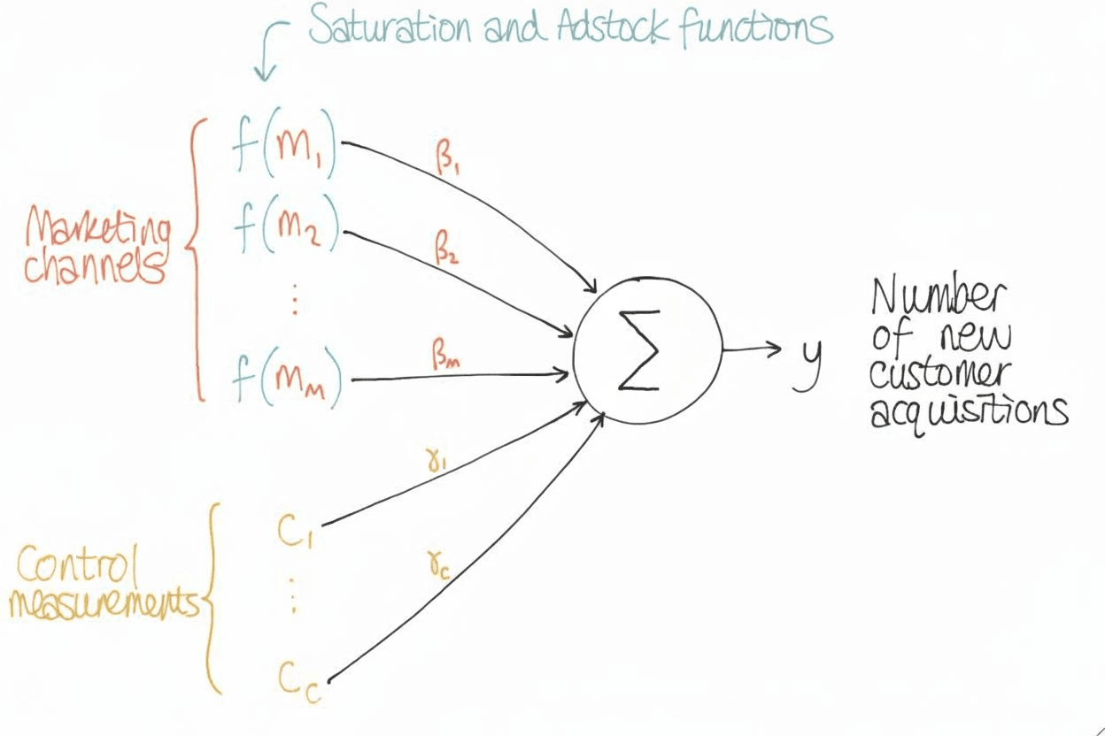
At the core of Marketing Mix Modeling is a regression equation that links sales with marketing activities and other factors. The simplest version looks like this:

Here's what each part means:

• Salest : Sales in week t
• TVt, Digitalt, Pricet, Seasonalityt : The independent variables, your inputs that can influence sales
• 1, 2, 3, 4:: Coefficients that measure the effect of each input on sales
• 0: Base sales, i.e., what you would expect to sell even without marketing
• t: Error term, the part of sales not explained by the model (random noise, unexpected events, etc.)

So, for example, if 1= 2.5, then every extra $1M spent on TV is associated with roughly $2.5M in additional sales, holding other factors constant.

This is the building block of MMM. In practice, we rarely stop here because marketing effects are not always linear or immediate. But this regression form gives us a starting point to split sales into base vs. incremental parts, compare channels, and plan budgets.

To see how regression and Bayesian modeling are applied in practice, take a look at our our talk at PyData on Solving Real-World Business Problems with Bayesian Modeling

Beyond the Basic Equation: Why Reality Isn’t Linear#

The regression model we just saw is a good starting point because it links sales with different marketing inputs in a clean, linear way. But real marketing effects are rarely that simple.

Spending on a channel doesn’t always translate to sales in a straight line. For example:

• If you spend $0 on TV, you get $0 impact. Fair enough.
• If you spend $10M, you see a lift in sales.
• But if you keep pouring money, say $1B on TV, sales don’t keep rising forever. People get saturated, ads lose effectiveness.

Timing also matters. A TV campaign may take weeks to build awareness, while digital ads can trigger responses almost instantly.

This is also where many MMMs can go wrong: if important factors are left out, the model can give biased estimates of how quickly returns diminish. In our post on Unobserved Confounders, ROAS and Lift Tests in Media Mix Models, we show how using lift tests as a “reality check” helps anchor these models and makes the saturation effect more trustworthy.

To handle this, MMM models don’t just stop at the basic equation, they add a few extra layers:

1. Adstock: to capture lag and carryover effects
2. Saturation: to model diminishing returns
3. Non- linear regression: to better reflect how marketing works in practice

We’ll dive into adstock and saturation next, but the main point is that MMM needs to reflect the messy, delayed, and diminishing nature of real-world marketing.

Adstock#

So far, our regression model assumes that the impact of advertising happens only in the week the money is spent. But in reality, that’s not how people behave.

If you run a TV ad on Sunday, not everyone buys on Monday. Some might buy that week, some a few weeks later, and some may forget altogether. In other words, the effect of an ad spreads over time and fades gradually.

To capture this, MMM uses a technique called adstock. Adstock creates a new version of your spend variable that accounts for this “carryover” effect. The formula looks like this:

That means the current effect is this week’s spend plus a fraction of last week, plus a smaller fraction of the week before, and so on.

For example, suppose you spend $1M on TV in Week 1 and nothing afterward, with λ = 0.8.

Week	TV Spend	Adstock (λ=0.8)
1	$1.0M	$1.0M
2	$0	$0.8M
3	$0	$0.64M
4	$0	$0.51M

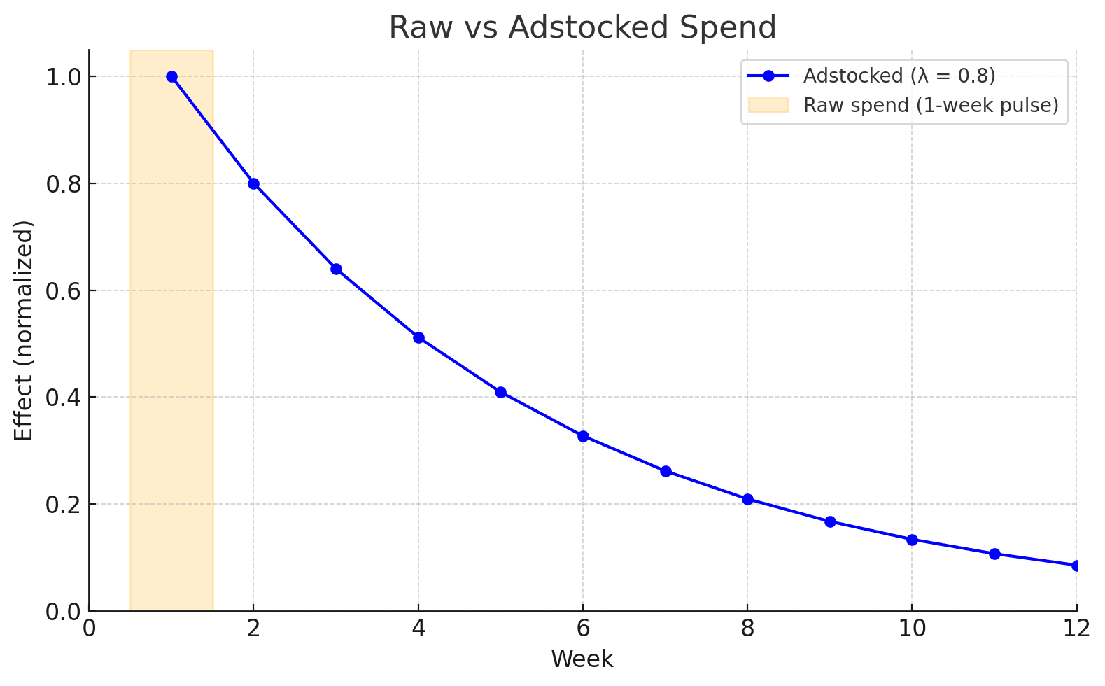
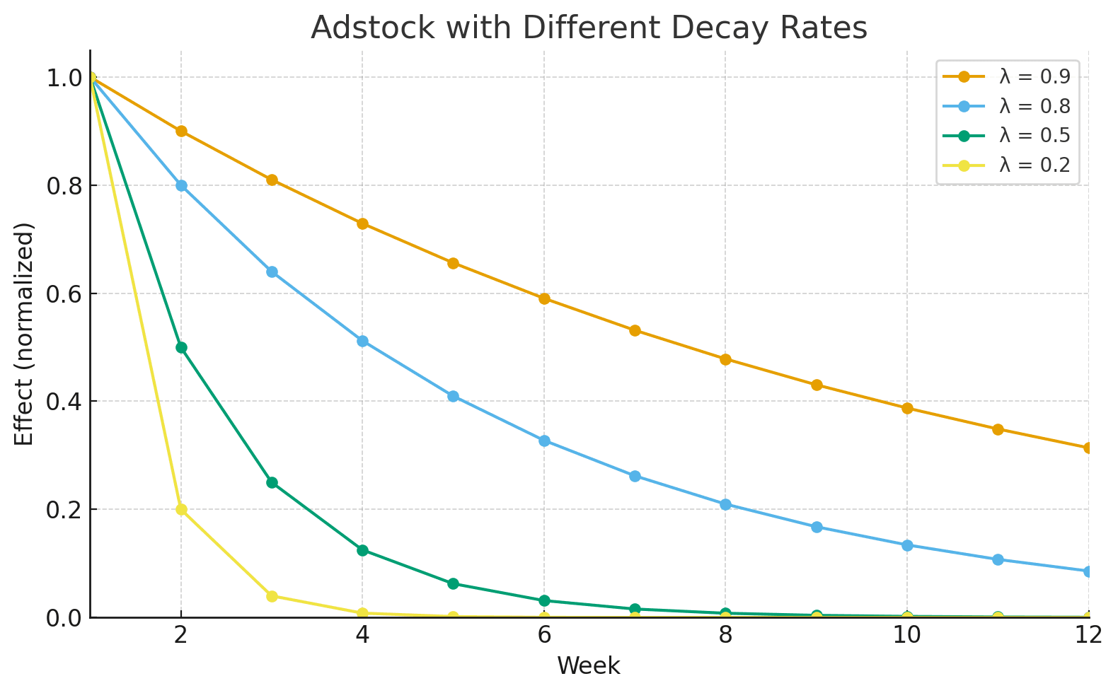
Since the spend carries over and fades slowly we use the adstocked spend instead of raw spend for TV, Digital and other channels

Saturation: Modeling Diminishing Returns#

Once we account for lag with adstock, there’s another challenge that is more spend doesn’t always mean proportionally more sales.

Eg:

• Week1: Spent $10K and we gained 1000 customers

• Week2: Spent $20K and we gained 1800 customers

• Week3: Spent $30K and we gained 2200 customers

You can notice here that, as the budget increases the customers gained isn't proportional. This is a classic example of diminishing returns.

Intuitively this makes sense because when you begin spending, the first part of your spend reaches the most responsive audience, and as you keep spending you end up reaching people who are hesitant, less interested, and harder to convince. So now, each dollar spent has less impact than initially.

To capture this MMM applies a saturation function to the adstocked spend before it enters regression.

Below are some saturation functions used:

1. Logarithmic function

• What this is saying is, at low spend, the curve grows steeply (high returns), but at high spend, it flattens out (diminishing returns).

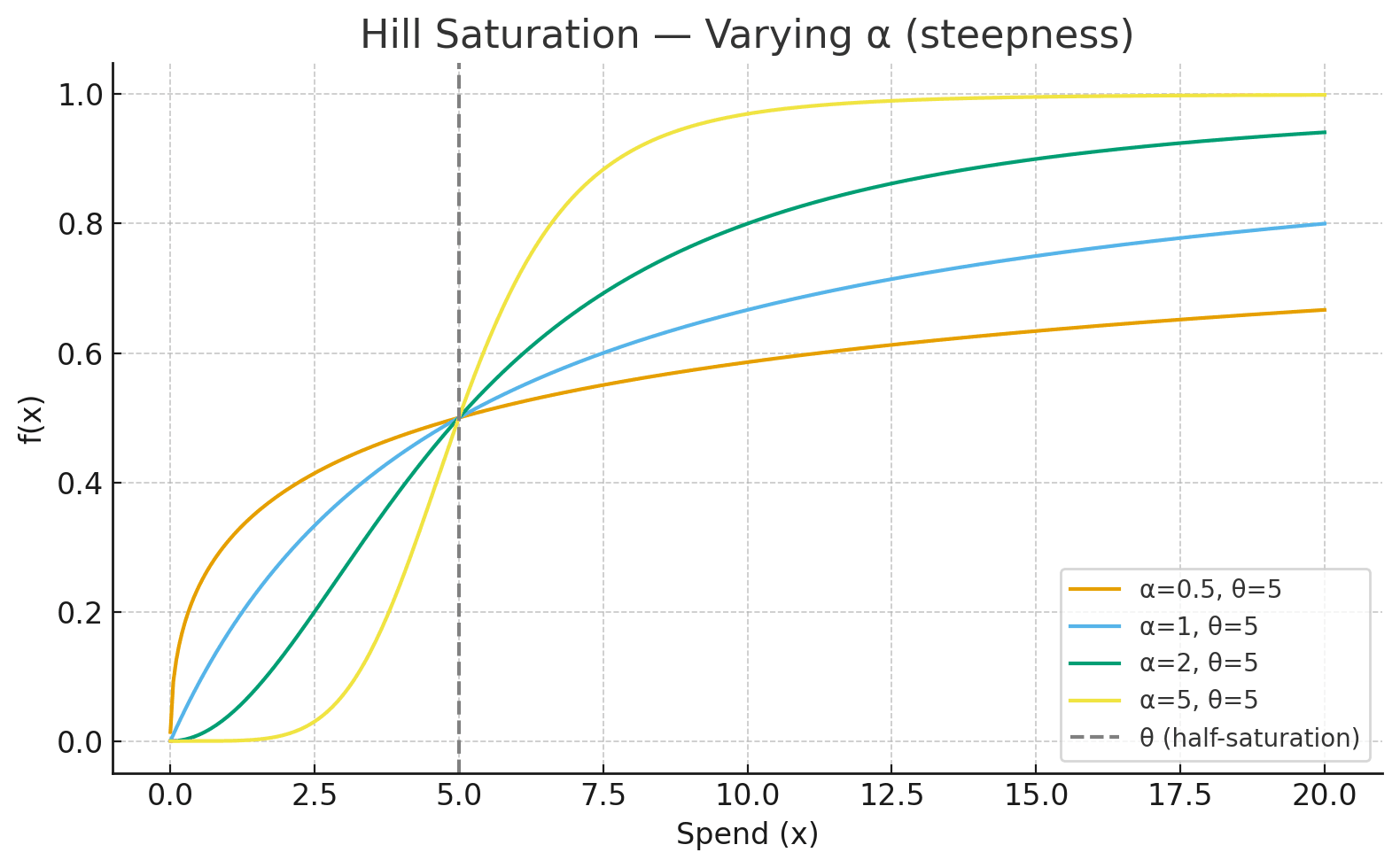
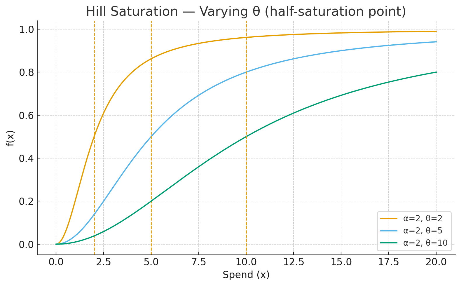
2. Hill function

• Here, controls steepness (how fast saturation occurs).
• is the half-saturation point (the amount of spend where the channel gives half of its total impact).

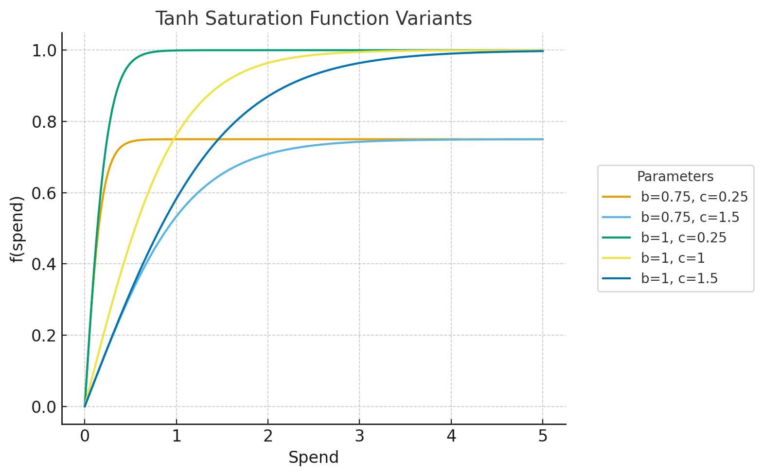
3. Tanh function

• is the ceiling, or the maximum possible impact the channel can deliver.
• controls the initial efficiency: smaller values make the curve climb faster (more customers per dollar at the start), larger values make it flatter (less efficient).

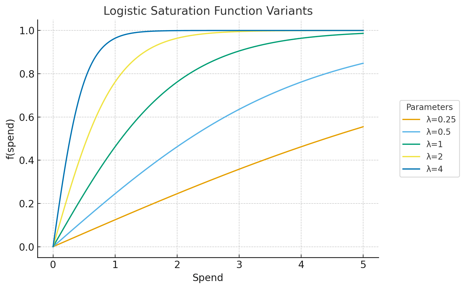
4. Logistic function

• controls efficiency. Larger values mean the curve rises faster (more efficient channel), while smaller values mean slower growth.
• The function has a half-saturation point at approximately , which makes it easy to interpret in business terms: “how much spend gets me halfway to the channel’s total impact.”
• Like and Hill, the curve is bounded: it rises quickly at first, then flattens smoothly as diminishing returns set in.

So now with adstock and saturation, our flow looks like this

In equation form we have:

where is the saturation function

Control Variables: Factors Outside Marketing#

So far we’ve looked at two big marketing behaviors, adstock and saturation. But if you think about it, marketing isn’t the only one that is moving sales up or down.

Sales can also shift because of non-marketing factors (nothing to do with ad spend) such as:

• A holiday like Christmas, creates spikes every year.
• Weather conditions, (eg: ice cream sales spike in summer heat)
• More shelf space for your product

These are called control variables. They’re not part of your marketing budget, but they still affect sales. If you leave them out, ads will get credit for changes they didn’t cause.

In practice, you just add them alongside your media channels to account for normal sales shifts things like seasonality, holidays, or competitor moves and separate those from the real incremental sales.

So now, our flow looks like this

Putting It All Together, The Full MMM Model#

So far, we’ve added layers, step by step, regression as the core, adstock to capture lag, saturation for diminishing returns, and control variables for non-marketing effects.

Now let’s see how they fit into one full model.

The equation looks like this:

Where:

• = spend on channel at time
• = carryover transformation as discussed
• = saturation function
• = effect of channel on incremental sales
• = control variables like holidays, weather, more shelf space, etc.
• = effect of those controls
• = error term (unobserved factors and noise)

Base vs. Incremental Sales#

Once this model is estimated, sales can be broken into two parts:

1. Base sales: what you’d expect with no marketing spend, driven by controls like price, holiday and trend.

2. Incremental sales, the extra sales generated by each marketing channel after adstock and saturation.

From Structure to Estimation: How Do We Find the Parameters?#

Until now, we’ve familiarized ourselves with the structure of an MMM. We have understood why we need adstock, saturation and control variables. But understanding and building this structure is just half the story.

The real challenge now is to find the parameters (the betas (β) , lambdas (λ) etc…)

This step is called parameter estimation.

For example, suppose we run our model and want to know: “How much does an extra $1M in TV spend improve sales?” If β (TV) turns out to be 2.5, we’d say that every $1M invested in TV drives roughly $2.5M in incremental sales. That’s the kind of answer estimation gives us.

There are two main ways to estimate these parameters: Frequentist and Bayesian.

The Frequentist Approach#

The classic way is Ordinary Least Squares (OLS) regression. Here’s how it works in plain terms:

1. You start with your historical data (sales, ad spend, prices, etc.).
2. The model makes predictions for sales given a set of coefficients (the β’s).
3. The “error” is the difference between predicted sales and actual sales.
4. OLS chooses the coefficients that make these errors as small as possible on average.

This gives you one best number for each parameter.

Frequentist methods are fast but have some important drawbacks:

• Point estimates only: You get one number for each coefficient (β(TV)= 2.5, say), without any sense of how uncertain that number is.
• Overconfidence: Real effects vary across markets, seasons, and contexts. A single number may oversimplify.
• Generalization risks: Frequentist models can struggle when data is sparse or noisy.
• Inability to include domain knowledge: Suppose you already know from past campaigns that digital ads usually decay faster than TV. In this approach you can’t directly encode that knowledge.

Bayesian methods are designed to solve these problems.

Why Bayesian Methods?#

Bayesian estimation replaces single “best guess” numbers with distributions. Instead of saying “TV adds exactly $2.5M,” Bayesian MMM might tell you:

• most likely between $2.0M and $3.0M
• but with some probability it could be lower or higher

This matters because it quantifies uncertainty rather than hiding it. At the same time, Bayesian methods give you all the strengths of Frequentist approach like clear parameter estimates and interpretability while also solving for the drawbacks. This is exactly what is needed for smarter decision making in MMM.

This shift matters because it quantifies uncertainty instead of hiding it, while still giving interpretable results. For a gentle intro to how Bayesian models do this, see MCMC Sampling for Dummies. And for a business view of why uncertainty is central, our blog From Uncertainty to Insight explains how Bayesian data science changes decision-making

What Marketing Mix Modeling Can (and Can’t) Do#

MMM is a reliable way to measure marketing impact, but it has its limits. It works best when you have a lot of historical data, which means it’s less useful for brand-new channels or sudden shifts in the market. Because MMM looks backward by design, it won’t give you instant answers on a new campaign. And since every model rests on assumptions, leaving out factors like competitor activity or shelf space can skew the results.

MMM also shines at the big picture more than the details. It can show you how TV or digital perform overall, but it won’t tell you if one specific ad drove sales on a Tuesday. And the more advanced the model, the harder it can be to explain outside of the data team, which sometimes slows adoption.

That’s why MMM works best alongside other tools like lift tests, incrementality experiments, and attribution. Together, they give you both the broad view and the finer detail.

…and this is where PyMC-Marketing steps in#

Everything we just discussed can be a lot to hand-code. PyMC-Marketing gives you a plug-and-play Bayesian MMM: adstock and saturation transforms, priors, MCMC fitting, posterior/HDIs, contributions, ROAS, forecasts, even budget simulations in a few lines.

Quick setup: channels, controls, transforms#

PyMC-Marketing wraps a full Bayesian MMM behind a simple API. You specify channels, controls, and pick your adstock + saturation.

from pymc_marketing.mmm import MMM, GeometricAdstock, LogisticSaturation

mmm = MMM(
    date_column="date_week",
    channel_columns=["tv", "digital"],
    control_columns=["price", "event", "t"],
    adstock=GeometricAdstock(l_max=8),
    saturation=LogisticSaturation()
)

Incorporate domain knowledge with priors easily#

You can add domain knowledge directly to your model with priors supported by pymc-extras. You just pick the priors that are relevant to you and PyMC-Marketing handles the rest.

from pymc_extras.prior import Prior

mmm = MMM(..., model_config={"adstock_alpha": Prior("Beta", alpha=1, beta=3)})

Model fitting made easy#

Model fitting is one line of code with mmm.fit( ), the package does all the heavy lifting so that you can focus interpreting results and less on debugging.

mmm.fit(X, y, chains=4, target_accept=0.9)

Prior-predictive check: validate assumptions#

You can test your priors before fitting the model by running a prior-predictive check. This lets you see if the priors you’ve chosen are reasonable or absurd.

mmm.sample_prior_predictive(X, y, samples=2000)
mmm.plot_prior_predictive(original_scale=True)

Model Diagnostics#

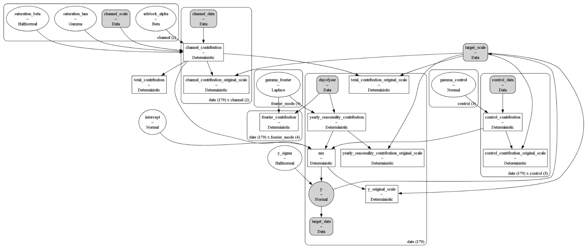
After fitting, PyMC-Marketing gives you diagnostics with ArviZ and a visual model graph. The graph helps you understand how your priors interacted with data and is a good way to confirm if your domain knowledge was included or not.

import arviz as az

az.summary(mmm_fit_result, var_names=["adstock_alpha", "saturation_lam"])
mmm.graphviz()

An example of model graph:

Posterior predictive: forecasts with uncertainty#

With PyMC-Marketing, forecasts don’t just give you a single number, they come with uncertainty bands. The result is easy-to-read “what if” scenarios where you see not just the most likely outcome, but also the range of plausible ones

mmm.sample_posterior_predictive(X, extend_idata=True, combined=True)
mmm.plot_posterior_predictive(original_scale=True)

Contribution decomposition#

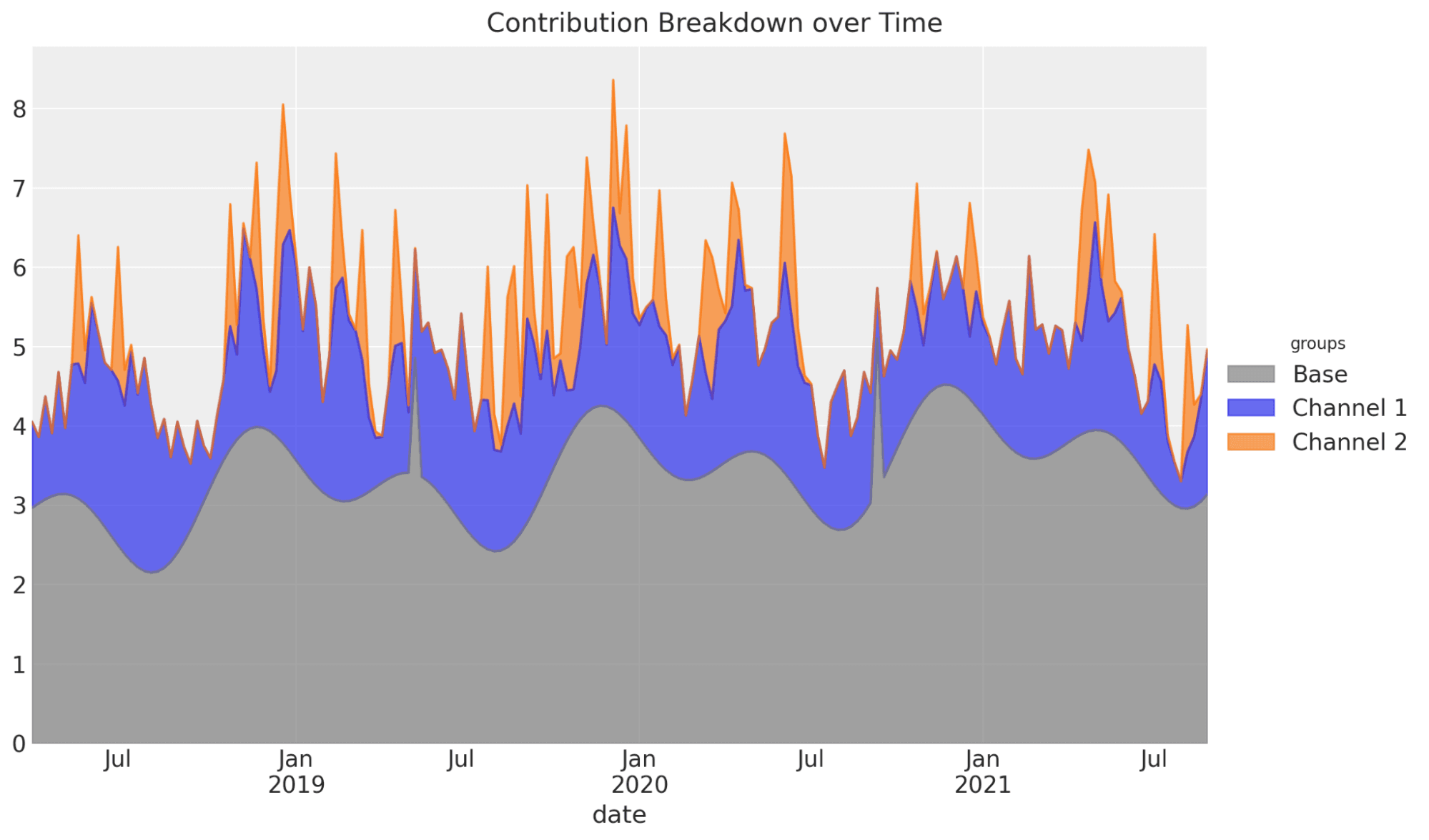
Remember we talked about figuring out the contribution of individual channels to sales? PyMC-Marketing shows how much each channel contributed to sales by separating baseline factors (trend, seasonality, controls) from channel lift, giving you a clear, business-aligned breakdown.

mmm.plot_components_contributions(original_scale=True)
fig = mmm.plot_grouped_contribution_breakdown_over_time(...)

An example of contribution breakdown over time:

Scenario curves and “what ifs”#

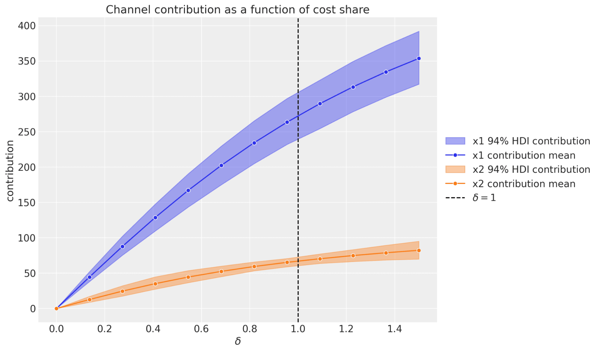
This feature is built right into PyMC-Marketing: you can quickly simulate what happens to contributions at different spend levels. The package generates curves that reflect adstock (carryover) and saturation (diminishing returns), guided by your priors.

mmm.plot_channel_contribution_grid(start=0, stop=1.5, num=12)

An example of channel contributions at different spend levels:

ROAS with uncertainty#

ROAS (Return on Ad Spend) isn’t shown as just one number. Instead, you get a range of possible values based on both your data and your priors. This makes the results more realistic especially when spend or data are limited and gives you a clearer picture of how much sales you’re actually getting back for each dollar spent.

chan = mmm.compute_channel_contribution_original_scale()
spend = X[["tv", "digital"]].sum().to_numpy()
roas_samples = chan.sum(dim="date") / spend[np.newaxis, np.newaxis, :]

Out-of-sample forecasts#

You can project sales beyond your data. Priors make sure ad effects fade out realistically instead of dropping off suddenly at the forecast horizon.

mmm.sample_posterior_predictive(X_oos, include_last_observations=True)

There are plenty more features too. The library also lets you add seasonality and trends, inspect parameters like adstock or saturation, and see channel shares with uncertainty. You can bring in lift test results to guide the model, use a time-varying baseline when markets shift, and save or reload models to keep things consistent over time.

In short, PyMC-Marketing gives you the full Bayesian MMM workflow from contributions and ROAS to forecasts and what-if scenarios while keeping priors and domain knowledge at the center.

What other open-source MMM tools exist?#

While PyMC-Marketing has gained a lot of traction, it's not the only open-source library available for Marketing Mix Modeling. Over the last few years, several major players including Google, Meta, and Uber have released their own approaches.

Each framework takes a slightly different path, some lean on more traditional regression techniques, while others emphasize Bayesian methods and advanced time-series forecasting.

The choice of tool often comes down to your team's technical expertise, the ecosystem you're already invested in, and how much flexibility you need for customization.

Here's a side-by-side comparison of the most popular options.

(Last updated: 2025-08-07)
*Meridian has been released as successor of Lightweight-MMM, which has been deprecated by Google

Feature	PyMC-Marketing	Robyn	Orbit KTR	Meridian*
Language	Python	R	Python	Python
Approach	Bayesian	Traditional ML	Bayesian	Bayesian
Foundation	PyMC	–	STAN/Pyro	TensorFlow Probability
Company	PyMC Labs	Meta	Uber	Google
Open source	✅	✅	✅	✅
Model Building	🛠 Build	🛠 Build	🛠 Build	🛠 Build
Out-of-Sample Forecast	✅	❌	✅	❌
Budget Optimizer	✅	✅	❌	✅
Time-Varying Intercept	✅	❌	✅	✅
Time-Varying Coeffs	✅	❌	✅	❌
Custom Priors	✅	❌	❌	✅
Custom Model Terms	✅	❌	❌	❌
Lift-Test Calibration	✅	✅	❌	✅
Geographic Modeling	✅	❌	❌	✅
Unit-Tested	✅	❌	✅	✅
MLFlow Integration	✅	❌	❌	✅
GPU Sampling Accel.	✅	–	❌	✅
Consulting Support	Provided by Authors	Third-party agency	Third-party agency	Third-party agency

If you are interested in a head-to-head benchmark between PyMC-Marketing and Google’s Meridian, check out our deep-dive blog PyMC-Marketing vs. Meridian: A Quantitative Comparison of Open Source MMM Libraries. The study shows PyMC-Marketing to be faster (2–20x), more accurate, and more scalable, thanks to its flexible sampler options.

Which open-source MMM library is the most popular today?#

Most open-source MMM libraries are built on Bayesian foundations, but they differ in how flexible they are, the tech stack they run on, and how they’re implemented.

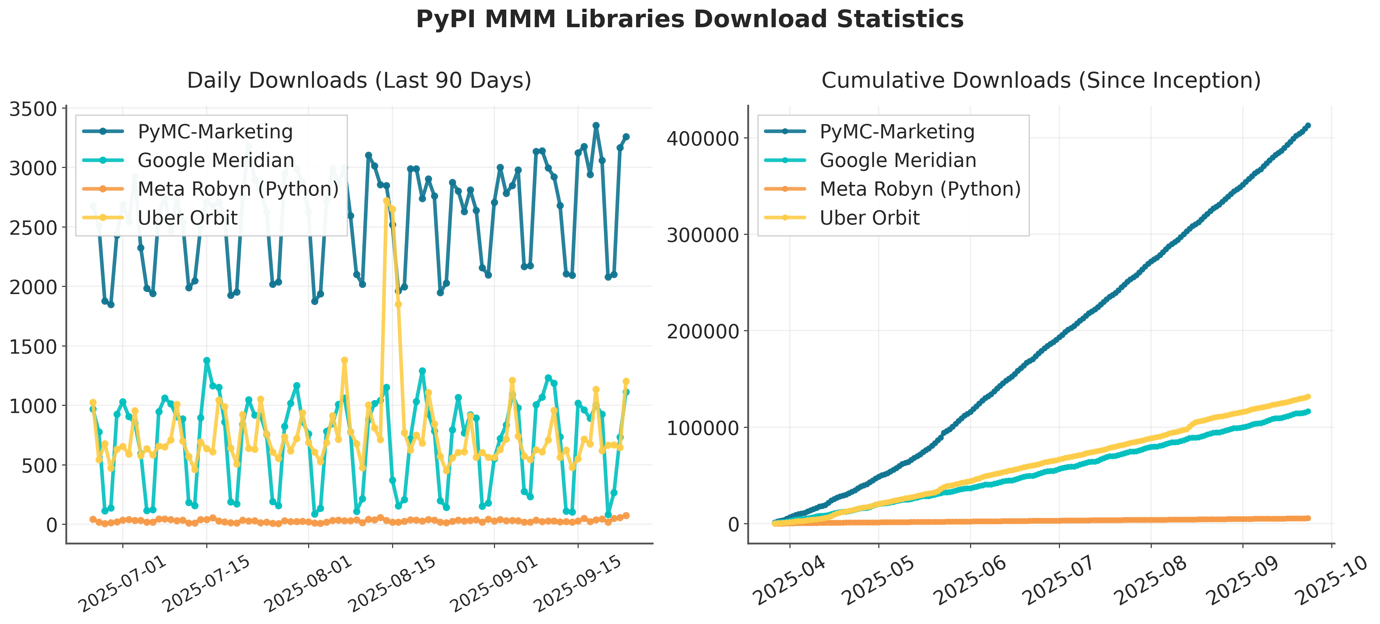
PyMC-Marketing has emerged as the most popular option by far, leading PyPI downloads (see chart below). It offers the widest feature set and the greatest flexibility, making it well suited for teams that need a customizable, state-of-the-art solution. The trade-off is that it’s also the most sophisticated, which can mean a steeper learning curve.

Other libraries fill different needs. Google Meridian provides a more opinionated API and integrates tightly with the Google ecosystem, which is useful for advertisers already working heavily in Google Ads. Meta Robyn, meanwhile, takes a more traditional regression approach and is a strong fit for teams using R that want a faster, simpler setup.

Your choice ultimately depends on:

• Your team’s technical expertise
• Your core advertising channels
• Whether you prefer an independent open-source solution or one backed by an ad network.

Which MMM library should you use? (Our Recommendation)#

The best tool depends on your team’s skills, your ad ecosystem, and how much flexibility you need. Here’s how we see it:

PyMC-Marketing

• Ideal if you need maximum flexibility for complex, unique business requirements.
• Supports advanced Bayesian modeling (including Gaussian Processes) and full customization.
• Production-ready with integration into data science workflows (MLflow, Python ecosystem).
• You prefer independence from major ad publishers and networks
• Optional consulting support from the authors.

Google Meridian

• You want a simplified API (but less flexible) to build models across geographies.
• Direct integration with the Google advertising ecosystem is important
• You want strong integration with other Google products such as Colab

Robyn (Meta)

• If your team works in R instead of Python.
• You prefer a simpler but less rigorous approach than Bayesian Models (Ridge regression)
• You want direct integration with Meta/Facebook advertising data.

Where is MMM Used in the Real World?#

Over the years, we've helped companies across different industries implement Bayesian MMM at scale. Here's how these projects actually played out in practice.

HelloFresh: Scaling Bayesian MMM from Prototype to Production#

When HelloFresh first began experimenting with Bayesian Marketing Mix Models, it was less a polished system and more a late-night experiment. The team had come across Google’s MMM paper and translated the original Stan implementation into PyMC. After cross-checking the model with company data, the results quickly built credibility.

One early recommendation was to increase TV spend. The marketing team was skeptical, as TV felt expensive compared to digital channels. But they took the risk, and the following quarter turned out to be one of their best.

From Prototype to Production Challenges#

The original model ran for hours. They needed time-varying effects to capture how COVID impacted different channels. Some digital channels became super expensive, others became cheap as advertisers either pulled back or concentrated everything into specific media.

Around this time, HelloFresh's work had caught attention at PyMCon 2020, where their MMM presentation was one of the most popular talks. That's how the collaboration with PyMC Labs started

The Technical Transformation#

Together, HelloFresh and PyMC Labs tackled the core challenges. Through re-parameterization and optimization, runtimes were cut down from hours to just minutes. Gaussian Processes were introduced so channel effects could vary over time, and a hierarchical structure allowed related channels like Facebook and Instagram to share strength.

Most importantly, the insights were translated into usable tools: visual reports and a web-based simulator where marketers could play out "what if" budget scenarios and see the predicted impact on conversions.

Business Translation is Key#

The collaboration wasn’t just technical. The models were translated into insights and tools that marketing and finance teams could actually use. This combination of technical innovation and business translation is what made the project successful.

HelloFresh now runs Bayesian MMM in production, with marketers and finance using it directly in planning cycles. The work also fed improvements back into the open-source PyMC ecosystem, so the innovations benefit the broader community beyond HelloFresh.

How Bolt built smarter budgeting with PyMC-Marketing#

Bolt faced a familiar challenge: attribution models were no longer enough. With privacy changes and fragmented channels, they needed a way to understand the true incremental value of their marketing investments across both digital and offline media. That's where PyMC-Marketing became a core part of their in-house analytics toolkit.

Using the library's Bayesian MMM framework, Bolt's team built models that accounted for adstock (carry-over effects) and saturation (diminishing returns), giving them a realistic view of how spend in each channel translated to outcomes. They didn't stop at modeling though. Every result was validated against experiments and quasi-experiments such as Google's CausalImpact, so the MMM stayed grounded in reality.

With calibrated models in place, Bolt could do more than just measure. They contrasted response curves across channels, identified plateau points where additional spend no longer drove growth, and used these insights to design automated budget allocation strategies. In practice, this meant their system could adapt to different business goals - sometimes prioritizing market share growth at any cost, other times optimizing for profitability or efficiency.

The impact was twofold. First, marketing decisions became faster and more data-driven, with resource allocation tailored to each campaign's objectives. Second, the collaboration strengthened the open-source ecosystem: Bolt contributed back by opening a pull request to add their budget allocation approach to PyMC-Marketing, ensuring other teams could benefit from the same advances.

As Bolt summarized in their write-up:

PyMC has earned its place among Bolt's treasured toolkits, thanks to the malleability it offers in crafting models perfectly suited to our needs. Along the same vein, PyMC-Marketing offers a compelling edge in devising flexible yet standard MMMs, serving both as a springboard and a muse for our analyses.

The Future of Marketing Mix Models: From Measurement to Decision-Making#

Marketing Mix Modeling has always carried a reputation for being slow and a bit academic, something that happened in the back office long after campaigns were over.

That’s changing quickly. The next wave of MMM isn’t about dashboards that summarize the past; it’s about tools that shape decisions in real time.

Making MMM Faster with AI#

Anyone who’s built an MMM knows the bottlenecks: endless data prep, debates about adstock curves, and nights chasing down model diagnostics. The modeling itself isn’t the biggest challenge, it is everything around it.

That’s exactly what the AI MMM Agent is built to solve. Acting as a co-pilot, it automates the critical but repetitive steps: cleaning data, configuring the right Bayesian model, running diagnostics, and translating outputs into business-ready insights. What used to take months can now happen in a day.

The result isn’t just speed (though speed matters in fast-moving markets). It’s accessible. MMM shifts from being a once or twice a year project into an ongoing decision-support tool that marketers and finance teams can use in real time.

Extending MMM Thinking Beyond Media#

The second shift we’re seeing is MMM-style thinking applied outside of media planning altogether. With our AI Innovation Lab, we take the same approach but aim it upstream at product development.

Here, synthetic consumer panels test ideas like packaging, pricing, or messaging before launch. It’s the same logic,but instead of asking “does TV drive sales?” the question becomes “does this new design actually win over buyers?”

We’ve validated synthetic panels against real consumer responses, showing up to 90% accuracy in categories like oral care. Combined with AI agents that simulate expert review for feasibility and compliance, the Lab gives companies a way to pressure-test products and campaigns weeks before they hit shelves.

Closing the Loop Between Product and Marketing#

The real step change comes when these tools connect. MMM tells you which channels and creatives work; the Innovation Lab tells you which product concepts resonate. Put them together, and you get a closed-loop system where product and marketing no longer operate in silos.

This means teams can align on questions that cut across functions: What should we launch? How should we price it? And how should we market it? Instead of chasing separate answers, they can share evidence, iterate faster, and act with confidence.

Breaking down the wall between consumer research and marketing planning doesn’t just make processes faster; it makes decisions smarter. It gives brands a way to build products and campaigns that reinforce each other, turning MMM from a rearview tool into part of the innovation engine itself.

FAQs on Marketing Mix Modeling (MMM)#

Q: How much historical data is needed for MMM to be effective?
We recommend at least one to two years of consistent sales and spend data. This helps the model distinguish true marketing impact from recurring patterns such as seasonality or external events.

Q: Can MMM cover both online and offline channels?
Yes. MMM can integrate digital, TV, radio, print, and in-store activities into one framework, providing a single view of how all channels contribute to sales.

Q: How frequently should MMM models be updated?
Many organizations refresh their models quarterly, while others update more often in fast-changing markets. The right cadence depends on your industry, data availability, and planning cycles.

Q: Does MMM replace experiments and attribution models?
No. MMM provides a broad, long-term view of channel effectiveness, while experiments and attribution add granular, short-term evidence. Used together, they provide a more complete understanding of marketing performance.

Q: Do you offer consulting or expert support for MMM?
Yes. At PyMC Labs, we work directly with teams to design, implement, and scale Bayesian MMMs. This includes everything from setting up models with PyMC-Marketing to customizing them for unique business needs. If you’re interested in collaborating or want to explore how Bayesian MMM could work for your organization, feel free to contact us for more details.

Conclusion#

Marketing Mix Modeling is becoming an essential way to see what really drives sales when tracking every click isn’t possible. Using Bayesian methods with open-source tools makes it easier to measure the impact of each channel and to be upfront about the uncertainty in the results.

At PyMC Labs, we’ve helped teams move from early tests to MMM systems that guide real budget decisions. That shift shows MMM is no longer just about reporting on the past. It’s about helping companies plan ahead with evidence they can trust.

As marketing gets more complex and decisions need to be made faster, MMM is turning into a practical tool for action. With the right data and setup, it can connect marketing and finance and give businesses the clarity they need to spend smarter.