Causal sales analytics: A deep-dive on discrete choice modeling

Introduction

In our first post on causal sales analytics we outlined the problem of estimating the degree to which a new product's sales are incremental (i.e. sales from customers new to the category or sales taken from competitors) or cannibalistic (i.e. sales that would have gone to your own existing products). We also outlined a multivariate interrupted time series approach which could be used to address this problem. However, we saw that while it was elegant and potentially has use in simple markets, it was not going to help us in a complex consumer goods market.

In this post we will sketch the solution that we built for Colgate-Palmolive. This solution is based on the discrete choice modeling framework, which is a class of model that is widely used in marketing and economics to model consumer choice.

Our solution represents a significant advance in the state of the art in causal sales analytics, beyond what is available in any published discrete choice modeling literature. We are excited to share this with the community and to show off the capabilities of the team here at PyMC labs.

The causal sales analytics problem

For our particular problem, it is important to remember that our client was a manufacturer of consumer goods and not a retailer. This means that they do not have access to consumer-level sales data. Instead, they have access to aggregated sales data at the product level for both their and competitor products.

This highly aggregated sales data was one of the key challenges in this project. Not being able to directly observe individual consumer choices means that we have to infer the underlying consumer choice behavior from the aggregate sales data. This is a challenging problem.

Our goal was to produce a causal sales analytics model that could be used by our client to estimate the degree of incrementality or cannibalization of new product introductions. This would allow them to make better decisions about which products to launch and how to market them. As we identified in our first post, having a causal approach to this problem is key because we need to make counterfactual inferences. More specifically, we need to estimate the counterfactual sales of all products would have been if the new product had not been introduced. The difference between the actual outcome and the counterfactual outcome will give us an approximation to the causal impact of the new product introduction.

The data had an unbalanced panel structure -- there were timeseries for many products. Each row corresponded to a given time period and product. It was unbalanced because not all products were available for sale in all time periods.

The outcome variable in our dataset (one of the columns) was sales volume, or the number of units sold, aggregated at the product level. No consumer-level or store-level data was available.

The other columns contain the predictor variables, which include:

• Price: the price of the product
• ACV: All Commodity Volume approximates the availbility of the product in the market. This was an important predictor variable in our model - a product may be fantastic, but if it is not on the shelf, it will not sell.
• Date: The data were available at weekly resolution
• Brand: the brand of the product
• Manufacturer: the manufacturer of the product
• SKU: the product ID in the form of a Stock Keeping Unit

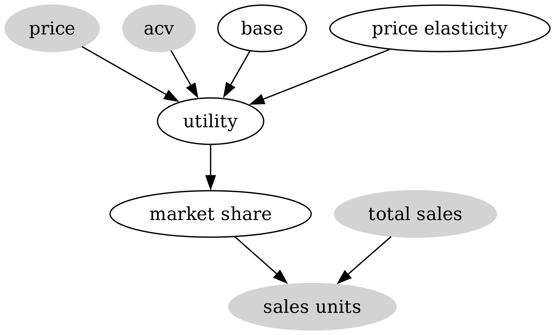
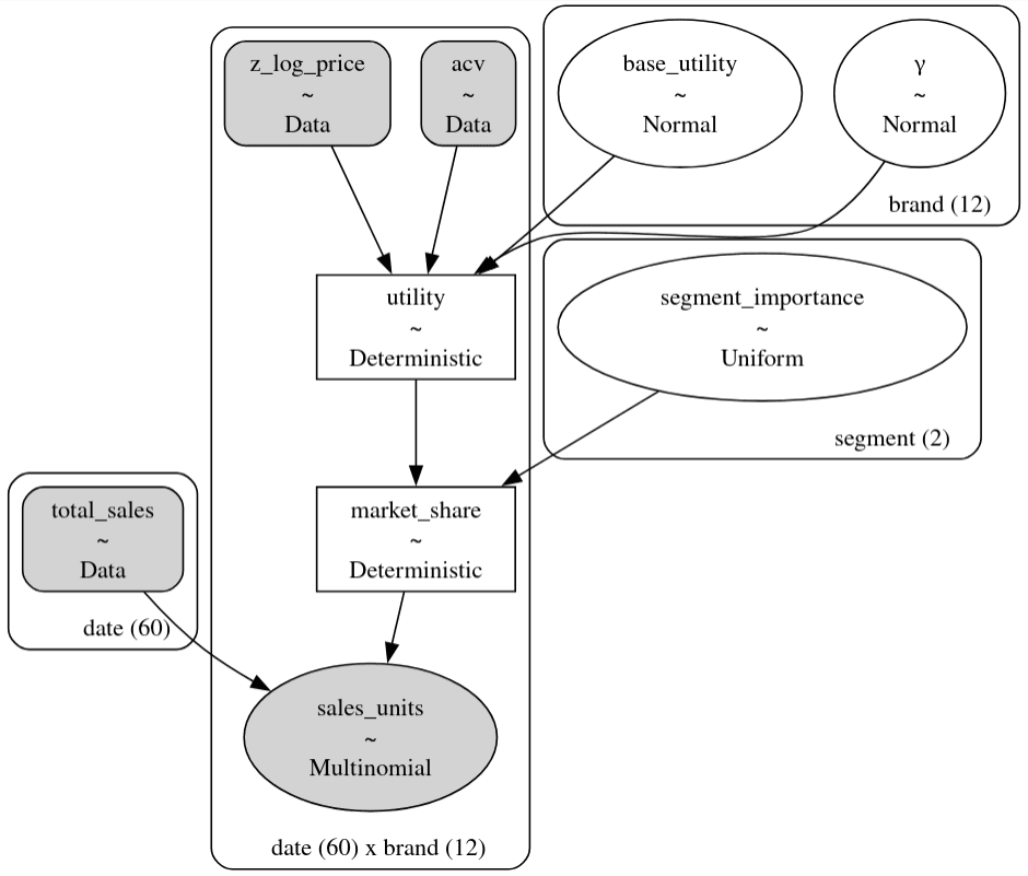
So let's put this together into a causal sales analytics model. Below we show one possible causal DAG describing the problem. We can describe this as:

• Price, ACV, base product appeal, and consumer price elasticity all causally influence the appeal (i.e. utility) of each product.
• The utility of each product causally determines its latent market share.
• The latent market share and the total sales demand causally determine the sales volume of each product.

Grey shaded nodes represent observed data, white nodes represent unobserved variables, and the arrows represent causal relationships.

A primer on discrete choice modeling

In this section we will introduce the basic approach by outlining a simple discrete choice model. This model is a vastly simplified version of what we built, but it will be sufficient to convey the general idea. We will highlight its limitations and, in a later section, we will outline our novel solution - both mathematically and computationally.

The core of our approach can be summarized as:

Individual consumers consider a menu of options (i.e. products) and choose that which maximizes their utility. Aggregate, market-level patterns reflect many individual choices.

Sales as a discrete choice problem

Our outcome variable (sales volume, or the number of units sold) is modeled as the outcome of rolling biased dice (i.e. total units), we can use a Multinomial likelihood function:

where is a vector with each value reflecting the number of times the corresponding product was purchased, is a vector with each value reflecting the probability each product is selected, and is the total number of purchases.

One may conceptualize as summarizing consumer preferences. So the question is, where do these preferences come from?

Utilities

Discrete choice models assume that consumers' choices reflect utility. Utility is a latent construct which, loosely speaking, captures how much an individual likes a particular option. The higher the utility of an option, the more likely the individual is to select that option. The lower the utility, the less likely the individual is to select that option. Utility is not directly observable, and thus must be inferred. The construct of utility has a long history in economics and can be a useful way to think about how people make choices.

How does this work? Discrete choice models assume that choice probabilities ( in the equation above) are a function of utilities. More specifically, we use the softmax function to convert utilities into probabilities :

where indexes the available products.

So, from the perspective of generalized linear modeling, the softmax is our inverse link function.

Where do utilities come from?

Simply put, we can use linear regression to create a mapping from product attributes to utilities. If we consider a single product, , then we can imagine that the utility of that product is a linear function of its attributes:

where:

• is the utility of product .
• is the intercept. We can interpret this as the baseline utility of product when all of its attributes are zero.
• is value of the th attribute of product .
• is the regression coefficient associated with the th attribute. We can interpret this as the change in utility brought about by a one unit change in attribute .
• is the error term. This is a random variable which captures the fact that we cannot perfectly predict the utility of a product from its attributes.

The approach outlined here will end up not being sufficiently flexible for the purpose of the current project. However, it is a good starting point for developing an understanding of discrete choice models.

!!! note "Product attributes are our predictor variables" Product attributes are the things which we think might influence the utility of a product such as price, brand, flavor, pack size, etc. For example, we might expect that the higher the price of a product, the lower the utility of that product, and therefore would expect price to be associated with a negative regression coefficient.

!!! note "Errors, " Different assumptions about the distribution of imply different choice functions. For example, if we assume then this leads to the logit/softmax approach. Alternatively, if we assumed were normally distributed then it would lead to the probit approach.

Simple discrete choice model in PyMC

Now that we've done a quick intro to discrete choice models, let's put it all together into code. Remember, this is a small toy example we are using to get acquainted with the general approach. Let's first take a look at a mathematical representation of the model:

We have observed data:

• : the all commodity volume of product at time
• : the price of product at time
• : the total number of sales at time

where is the index of the product and is the index of the time period.

The parameters are:

• : the base utility for a given item when all other predictors are zero. The higher this value, the more likely it is to be purchased, ignoring all other factors.
• : the price elasticity for item . Although bear in mind that this represents the % change in utility for a 1% change in price. This is not the same as the % change in sales for a 1% change in price.

The softmax function is computed over all products at time .

Bear in mind that we've modified the equation defining utility a bit. We've added a multiplicative effect of price upon utility which allows us to include a parameter that represents price elasticity, .

The term is how we dealt with products that are only partially available. For example, if an item's ACV is zero (it is not available for purchase anywhere), then the log will be negative infinity. This will make the item's utility negative infinity and the probability of that item being purchased will be zero.

Note that we are assuming that total sales are exogenous - that is, is provided to us as an observed quantity. In our actual client work, we modeled the data generating process that gave rise to total sales, but we will not cover that here.

Loading simulated data

We'll load some simulated data to illustrate this model.

data = pd.read_csv("dataset.csv", parse_dates=["date"])
data

product_df = data[["segment", "manufacturer", "brand"]].drop_duplicates()
product_df

Below we plot the data. The top plot shows that there are different "classes" of products. Some are persistently distributed throughout the time period we are looking at. Others are introduced, with availability starting at zero and ramping up. Finally, some are discontinued, with availability ramping down to zero. The second plot shows the price of the products, and the last two show the total sales and market share of each product.

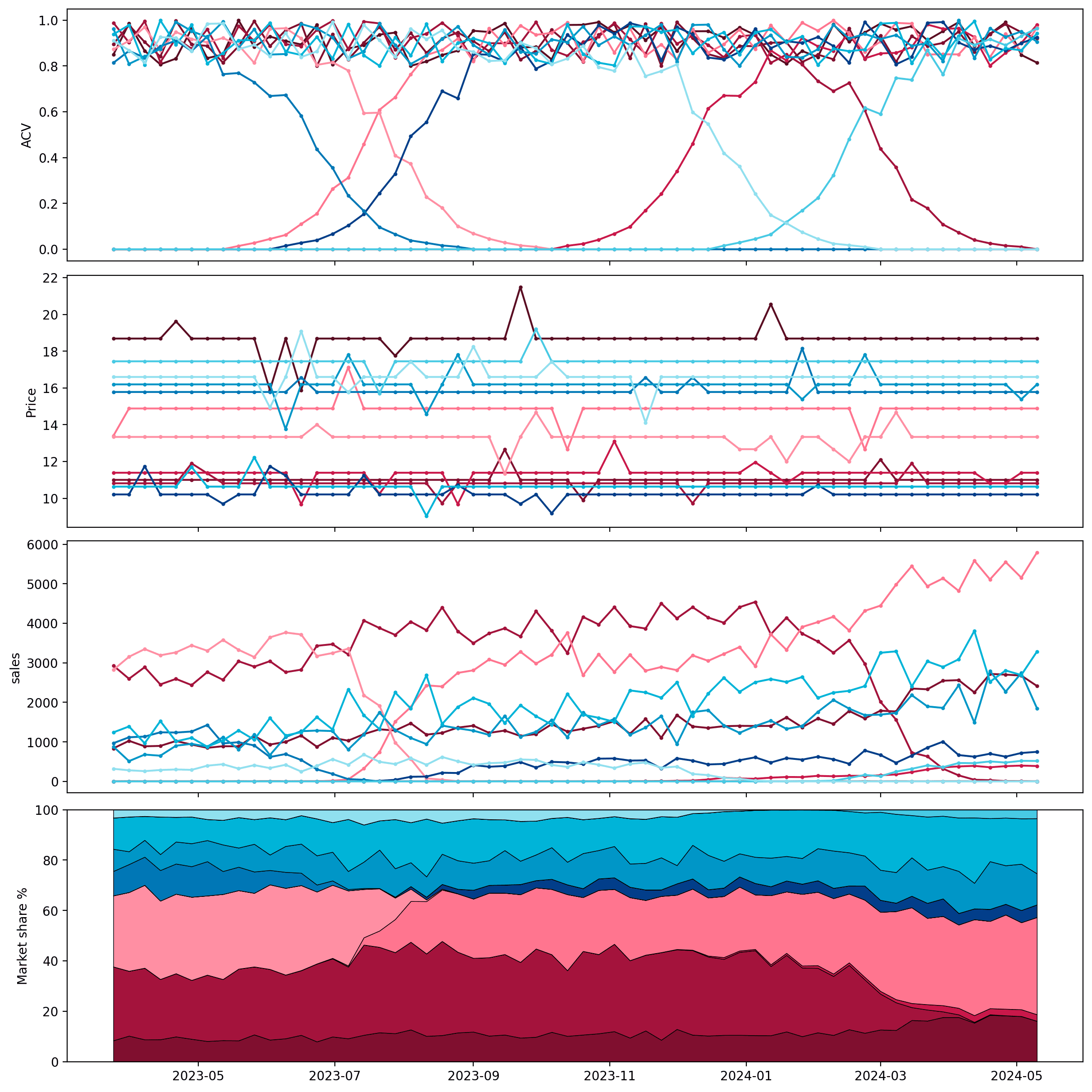
Products in blue belong to the first segment and products in red to the second.

Now we'll build the model in PyMC and fit this data.

coords = dict(
    brand=product_df["brand"].values,
    date=date,
)

with pm.Model(coords=coords) as simple_logit_model:
    # Data
    acv_data = pm.Data("acv", acv, dims=["date", "brand"])
    total_sales_data = pm.Data("total_sales", sales_units.sum(-1), dims=["date"])
    z_log_price_data = pm.Data("z_log_price", z_log_price, dims=["date", "brand"])

    # Priors
    base_utility = pm.ZeroSumNormal("base_utility", dims="brand")
    γ = pm.Normal("γ", mu=-0.8, sigma=0.2, dims="brand")

    # Model
    utility = pm.Deterministic(
        "utility",
        base_utility + pm.math.log(acv_data) + γ * z_log_price_data,
        dims=["date", "brand"],
    )

    market_share = pm.Deterministic(
        "market_share", pm.math.softmax(utility, axis=-1), dims=["date", "brand"]
    )

    # Likelihood
    pm.Multinomial(
        "sales_units",
        n=total_sales_data,
        p=market_share,
        dims=["date", "brand"],
        observed=sales_units,
    )

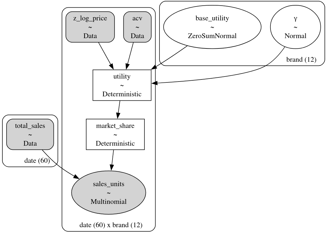
It always helps to understand a model by looking at its graphviz representation. We can see the direct similarity between this PyMC graphviz representation and our causal DAG above.

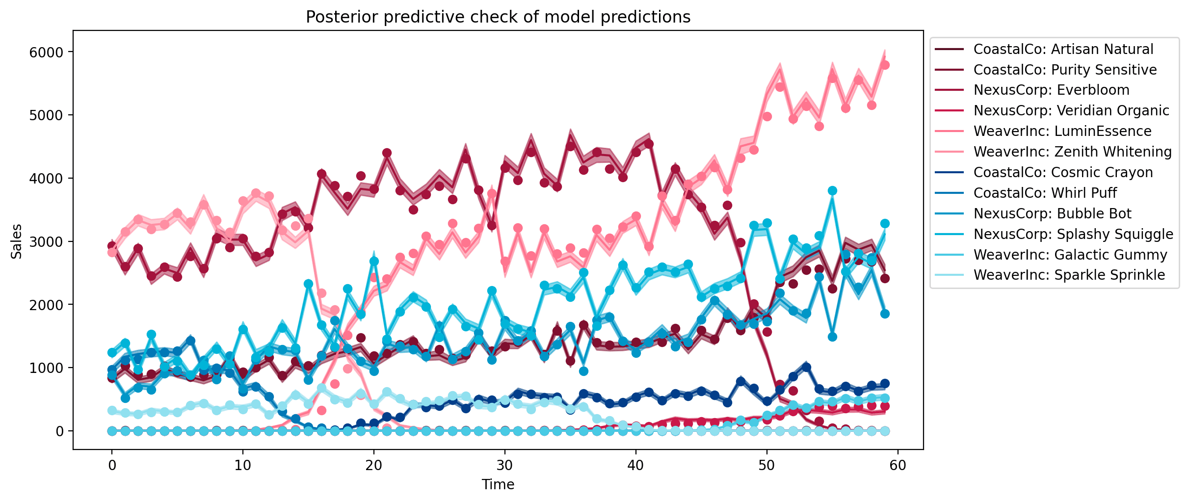
Let's check how well the model is able to account for the observed data. We'll do this by comparing the observed sales data (points) with the model's posterior predicted sales (lines represent posterior mean and shaded regions represent 94% HDI's).

with simple_logit_model:
    idata_simple_logit_model = pm.sample(random_seed=rng)
    pm.sample_posterior_predictive(
        idata_simple_logit_model, random_seed=rng, extend_inferencedata=True
    )
plot_post_pred(idata_simple_logit_model)

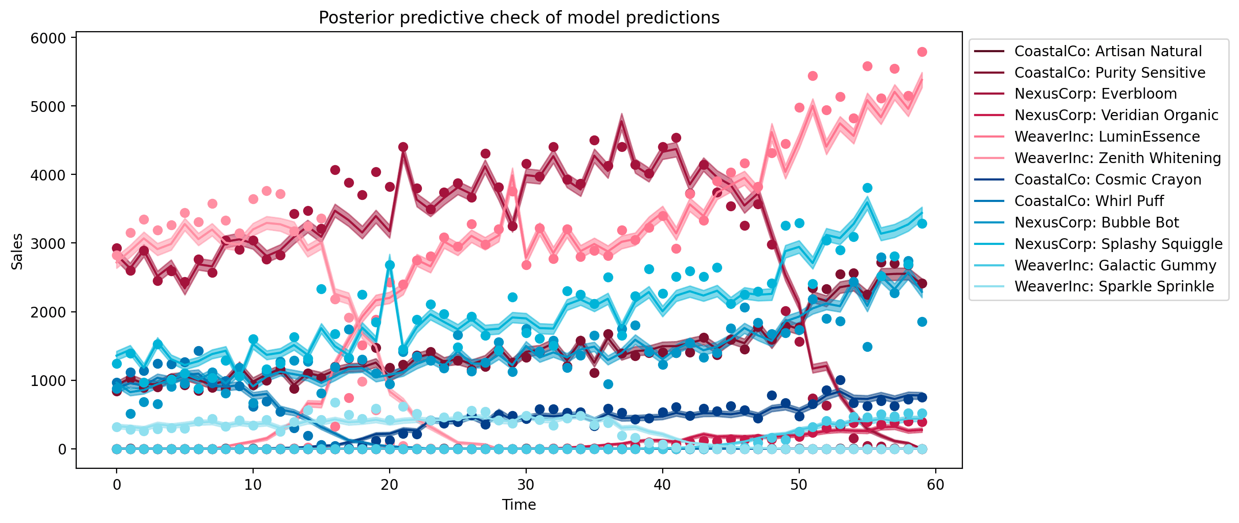
The model is doing an okay job at accounting for the general trends observed data, although the posterior distributions for the parameters often miss the true values.

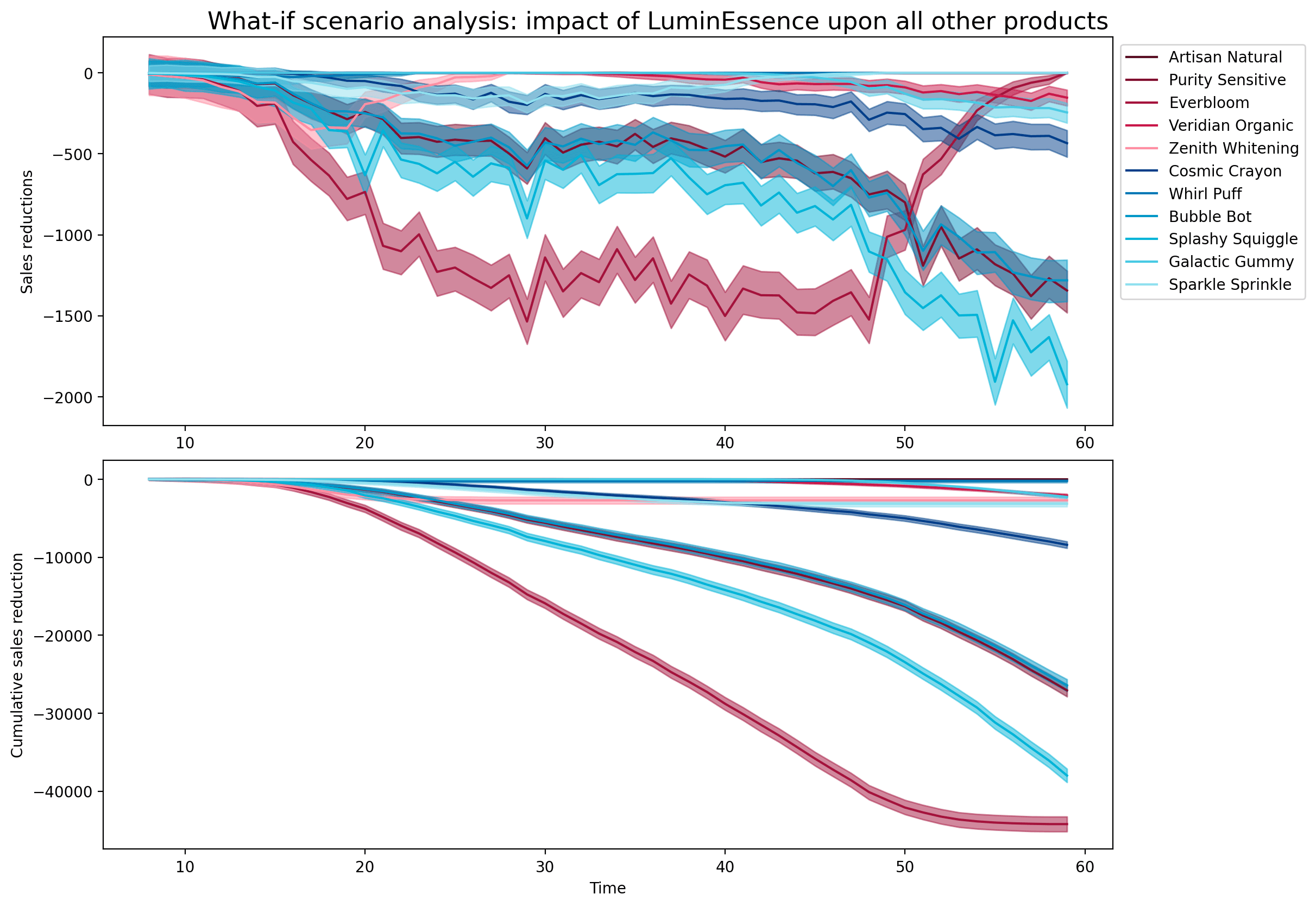
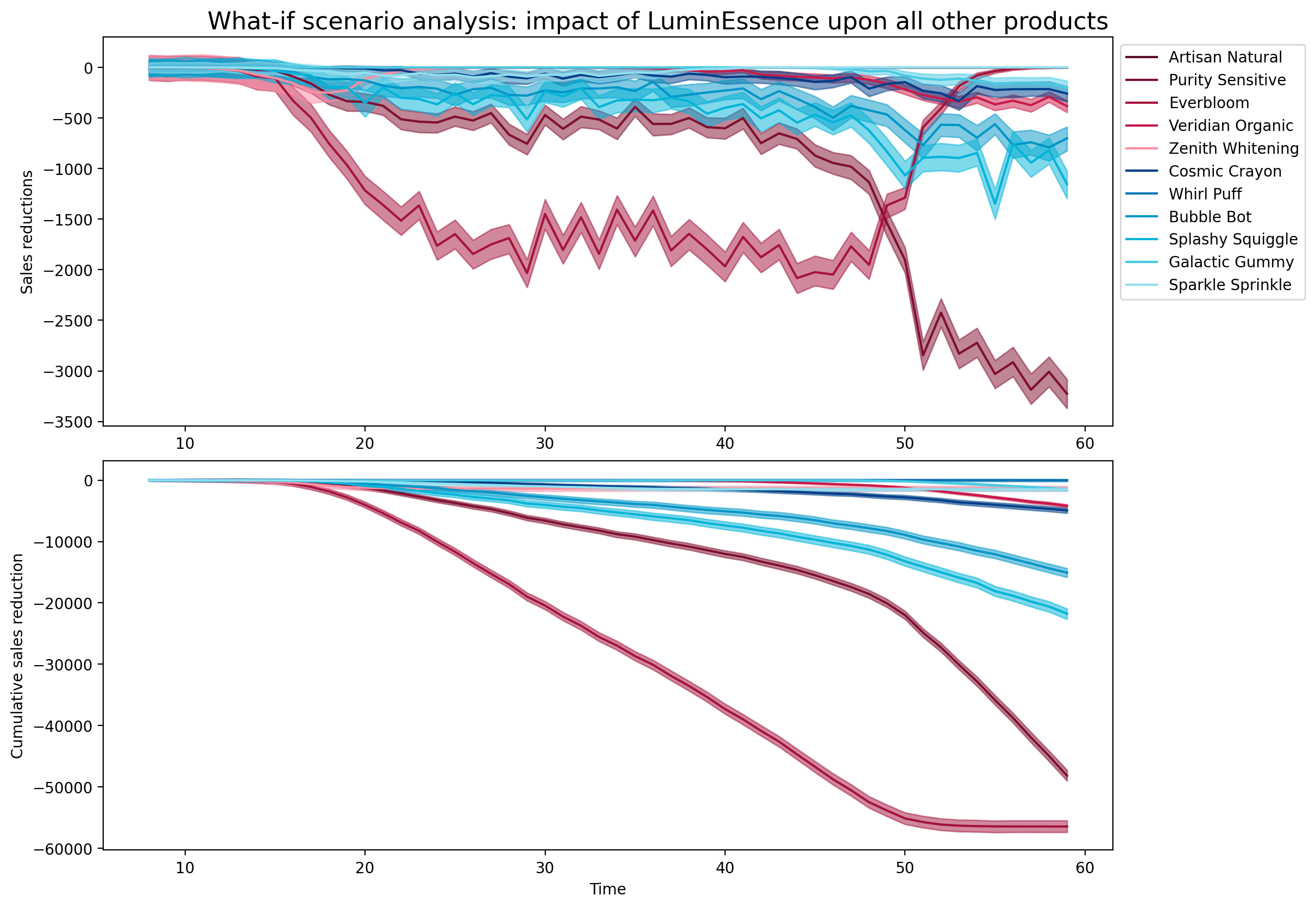
Exploring counterfactual scenarios

In this section, we'll put the causal in our causal sales analytics. We're going to look at one of the products that was introduced and estimate the causal impact its introduction had upon the sales of other products.

# remove a product so that it's one that was newly introduced during the time period.
brand_to_remove_idx = 4  # 3
brand_to_remove = product_df.iloc[brand_to_remove_idx]
brand_to_remove

# remove brand_to_remove_name from the list of items
remaining_brands = [
    brand
    for i, brand in enumerate(product_df["brand"].values)
    if i != brand_to_remove_idx
]

# create counterfactual ACV data
acv_counterfactual = np.copy(acv)
acv_counterfactual[:, brand_to_remove_idx] = 0.0

# find the index of the first date where acvs[:, product_to_kill] is > 0
first_non_zero = np.argmax(acv[:, brand_to_remove_idx] > 0)

# %%
# do posterior prediction under that counterfactual ACV scenario
with simple_logit_model:
    pm.set_data({"acv": acv_counterfactual})
    predictions = pm.sample_posterior_predictive(
        idata_simple_logit_model,
        var_names=["sales_units", "market_share"],
        predictions=True,
        random_seed=rng,
        extend_inferencedata=True,
    ).predictions

# %%
plot_causal_impact(idata_simple_logit_model, brand_to_remove_idx, brand_to_remove)

Limitations of the basic discrete choice model

So far, so good. We've got a setup where:

• We have a model that links availability (ACV) and price data to sales volumes.
• It estimates base utilities and price elasticities for each product.
• It can be used to estimate the causal impact of new product introductions.
• We can estimate the causal impact on own vs other manufacturer products, estimating the level of cannibalization and incrementality, respectively.

So what's the catch?

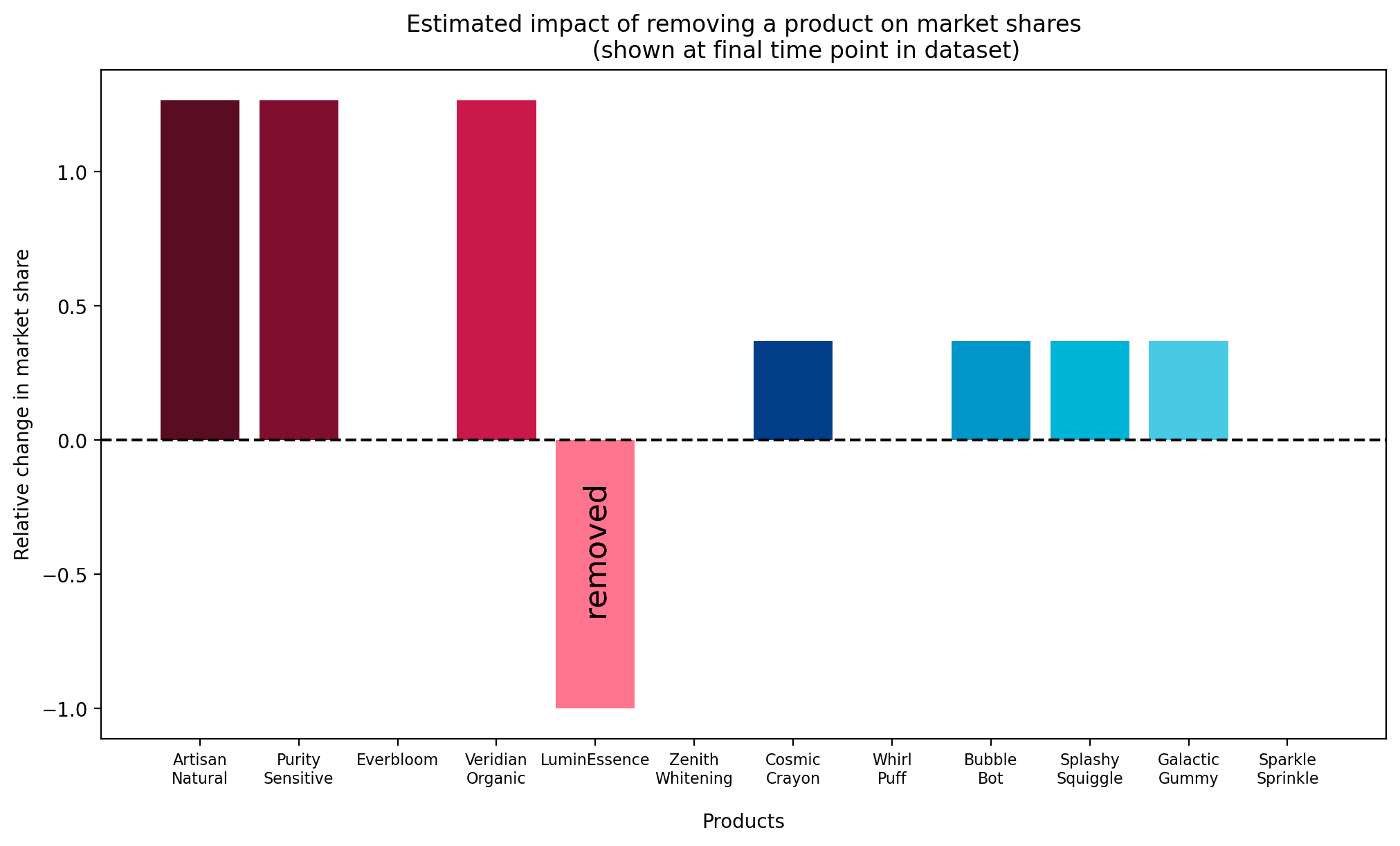
The catch is that this model is incapable of generating "interesting" patterns of cannibalisation. What we mean by this is that in our counterfactual scenario, the scenario in which we consider what would have happened had a product never been introduced, the model will predict that the market share of the all remaining products increase proportionally.

We can demonstrate this by plotting the posterior relative change in market_share at a specific date, and noting that it is the identical for all items:

plot_last_day_rel_market_share_change(idata_simple_logit_model, brand_to_remove_idx)

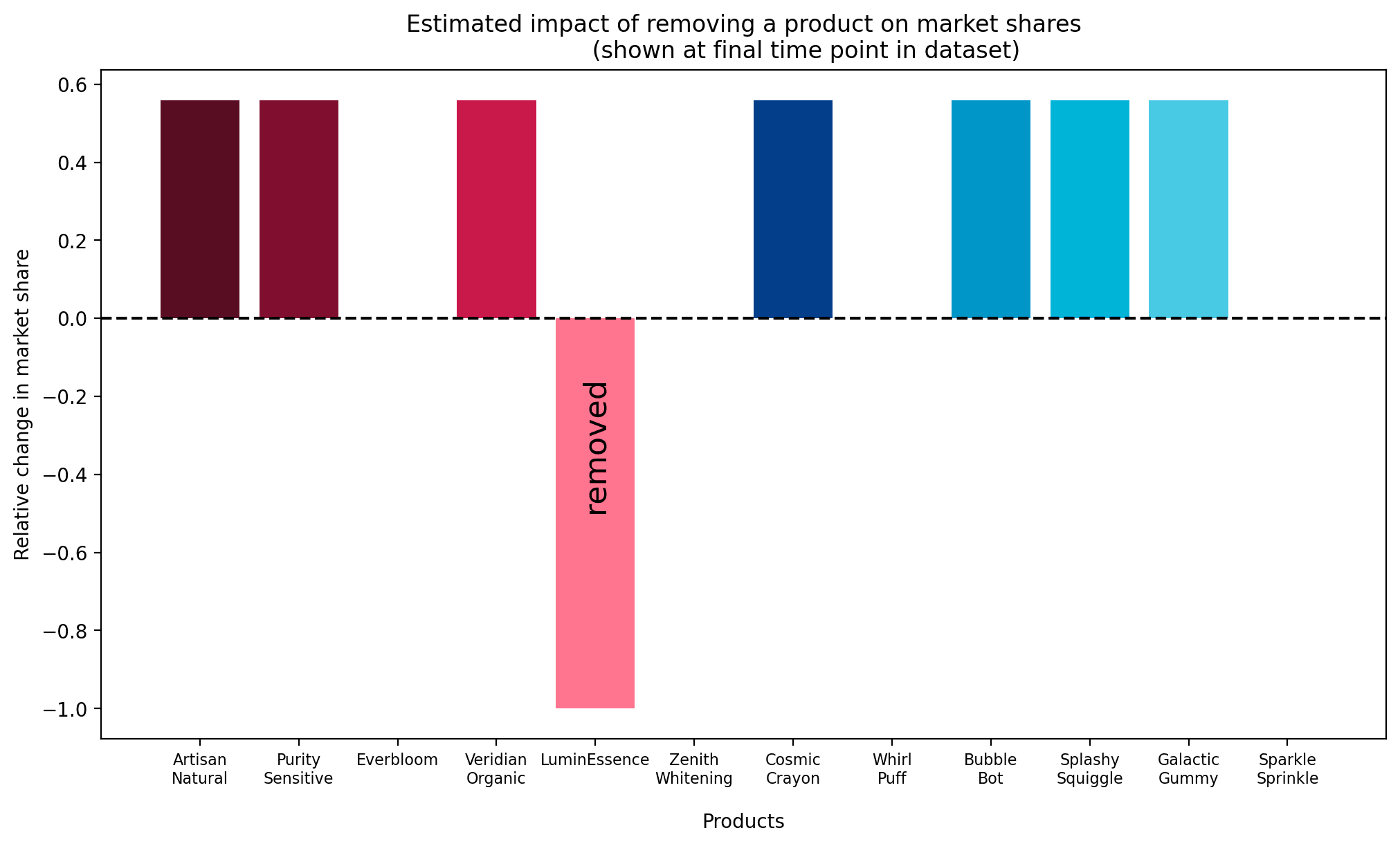
This is almost certainly not what we would expect to see in the real world.

For example, if the newly introduced product was marketed in the "kids" segment, we might expect it to take sales from other products in that category, but not (as much) from other categories such as "adult" segment. This is a more complex pattern of cannibalization than the current model is capable of capturing.

So despite the fact that this model has many strengths, the inability to accurately capture realistic cannibalization patterns is a significant drawback. It is this limitation that pushed us to develop a more advanced model for our client.

What's missing

Our intuition tells us that there is some key factor that is driving people's choices but absent from our model. For example, having children in a household creates a specific need for "kid-friendly" toothpaste. If one "kid-friendly" item is removed from the shelf, customers that previously purchased it will not pick any random toothpaste as a substitute. They will almost certainly switch to another "kid-friendly" item.

We have no hope of getting this sort of individual-level information from our dataset of global sales, and even if we had, it would be extremely hard to figure out how to leverage it explicitly. We'll leave it to statistical inference to work out those details.

We briefly mentioned the role of the model "error term" as a catch-all bucket for "information we don't have". It's a placeholder for all the personal, hidden reasons a customer makes a choice that aren't explicitly modeled. This includes things like having kids or cavities, as well as more distal causes such as being in a hurry on a day or having a store coupon for a specific item. The simple logit model assumed these unknowns were not correlated across different items. It assumed that the personal reasons leading a customer to purchase "KidsShine" were entirely unrelated to the reasons leading a customer to purchase "AquaBuddies".

Let us refine this assumption, using a well-researched model that we developed for Colgate-Palmolive: the nested logit model.

Nested logit discrete choice model

The nested logit model is, in essence, a series of simple logit models glued together hierarchically, in a way that still respects the idea of utility maximization.

Items are grouped into distinct nests, representing things like "segment" and "brand", that we hope will capture the relevant but unobserved factors driving consumer choices. Ideally, pairs of items within the same nest will share important factors such as being kid-friendly, whereas items from distinct nests will only share less-predictive factors like being closer to the store entrance (e.g., to be grabbed by consumer in a hurry).

Statistically, the nested logit model will expect errors to be correlated within nests and, subsequently, predict preferential substitution patterns within items of the same nest.

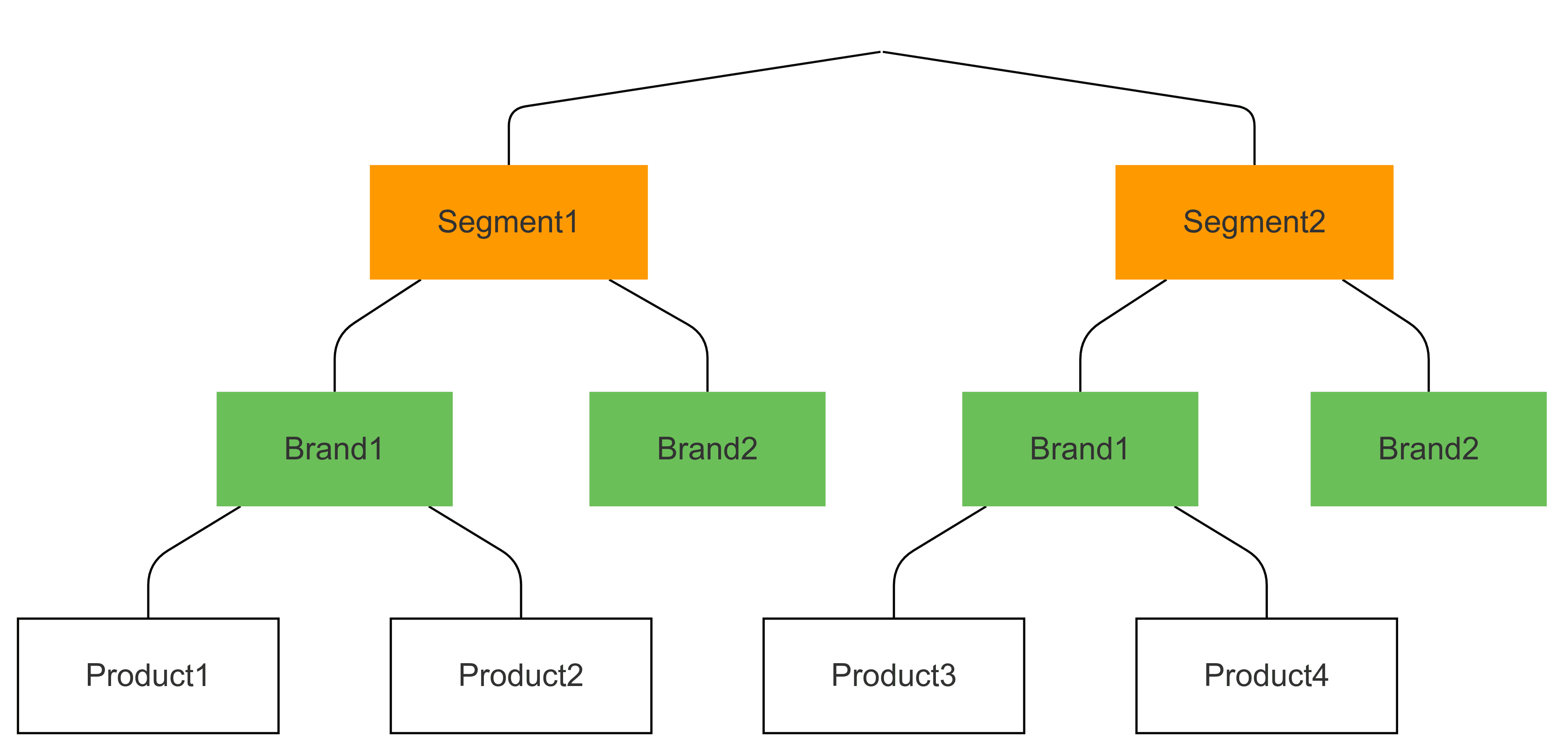
Furthermore, nests can be ordered hierarchically. We may believe items of the same brand within the same segment share more choice-relevant characteristics than items of the same brand in different segments. This would mean, we believe in a "segment -> brand" hierarchy. As we move down the hierarchy, substitution patterns will increase in strength.

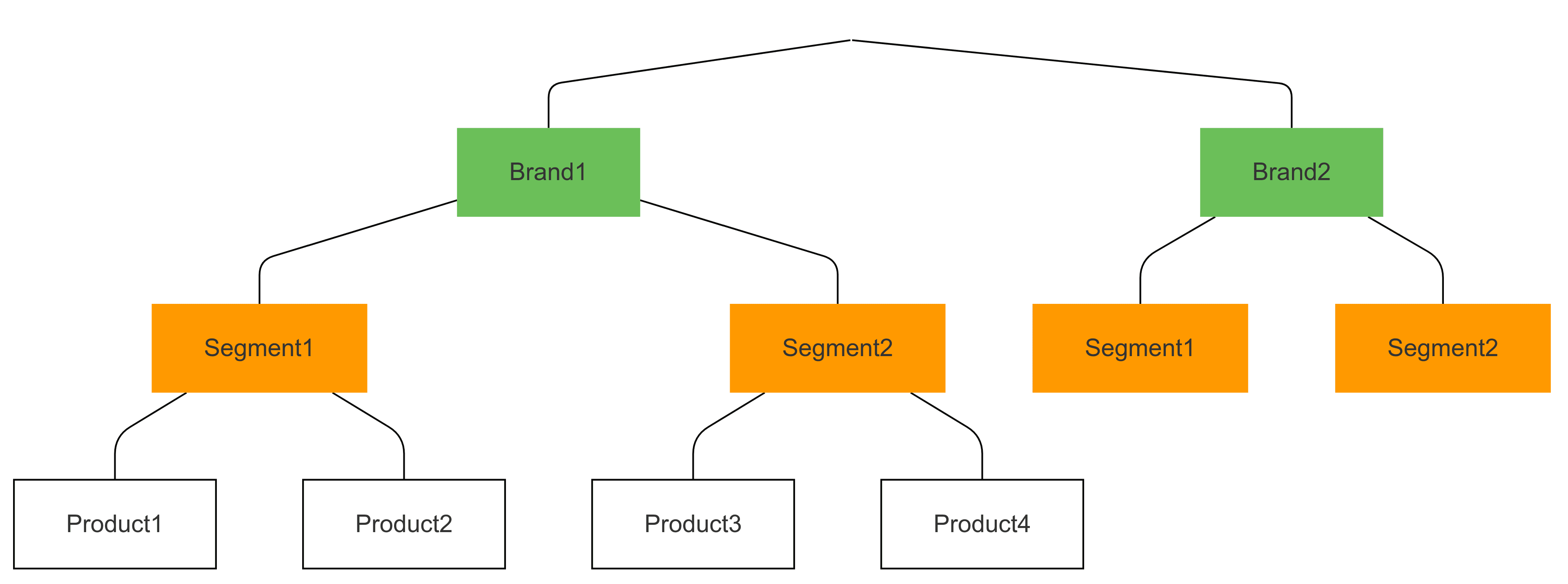
Alternatively, if brand is a much stronger driver of choice than segment is, we might define a "brand -> segment" model, where we believe cannibalization will be much stronger across segments of the same brand, than across brands of the same segment.

The nested logit model allows us to study this sort of nuance!

The math

Let's briefly discuss how the nested logit models works from a mathematical point of view. The nested logit model computes the overall probability of choosing an alternative as the product of:

1. the probability of choosing a nest (marginal probability)
2. the probability of choosing an alternative within that nest (conditional probability, given that nest)

The nested logit probability can be written as the probability of choosing a particular nest and then the conditional probability of choosing a product within that nest:

To keep things concise we will only consider one level of the hierarchy: segment.

Our utility will remain roughly the same as in the case of the simple logit model above, except now there are two contributions to the utility of a product: The product-specific contributions, and a aggregate of the contributions of items from the same segment,

Specifically:

This tells us, that conditional on a given nest, only the product-specific utilities, , play a role (scaled by a shared ). This is a simple logit model.

and

where

Therefore, the probability of choosing a specific nest is a function of all the product-specific utilities in each nest, scaled by an "importance factor",

We won't delve too much on the meaning of . For our purposes we can think of it as a loose knob that determines the degree to which items in a nest have preferential substitution.

PyMC implementation

We developed some state-of-the-art tooling to extend the nested logit model to arbitrary levels of depth, while keeping it performant and numerically stable. We have also developed semi-automated specifications for the priors over nest importances, so that the model remains consistent with utility maximization theory.

This is critical because real-world products are often characterized by a wide variety of attributes (e.g., brand, sub-brand, segment, sub-segment, organic or not, flavor, color, packaging format, etc.) and brands invest heavily consumer insights/market research units that strive to understand exactly how consumers arrive and their final decisions. As a result, brands can easily construct extremely deep (and wide) nestings in order to characterize offerings available on the market.

coords = dict(
    brand=product_df["brand"].to_list(),
    segment=product_df["segment"].unique(),
    date=date,
)

with pm.Model(coords=coords) as nested_logit_model:
    # Data
    acv_data = pm.Data("acv", acv, dims=["date", "brand"])
    total_sales_data = pm.Data("total_sales", sales_units.sum(-1), dims=["date"])
    z_log_price_data = pm.Data("z_log_price", z_log_price, dims=["date", "brand"])

    # Priors
    γ = pm.Normal("γ", mu=-0.8, sigma=0.2, dims="brand")
    base_utility = pm.Normal("base_utility", dims="brand")

    # Model
    utility = pm.Deterministic(
        "utility",
        base_utility + pm.math.log(acv_data) + γ * z_log_price_data,
        dims=["date", "brand"],
    )

    segment_importance = pm.Uniform("segment_importance", dims="segment")

    # Modify utility according to one-level NLM
    idxs = np.array([0, 0, 0, 0, 0, 0, 1, 1, 1, 1, 1, 1])
    # Need to fudge the utility to avoid divide by zero errors when acv=0
    utility_brand_given_segment = pm.math.exp(
        pm.math.clip(utility, -300, utility) / (1 - segment_importance)[idxs]
    )
    sum_utility_brand_per_segment = pm.math.concatenate(
        [
            utility_brand_given_segment[:, :6].sum(axis=-1, keepdims=True),
            utility_brand_given_segment[:, 6:].sum(axis=-1, keepdims=True),
        ],
        axis=1,
    )
    p_brand_given_segment = (
        utility_brand_given_segment / sum_utility_brand_per_segment[:, idxs]
    )
    util_segment = pm.math.exp(
        pm.math.log(sum_utility_brand_per_segment) * (1 - segment_importance)
    )
    p_segment = util_segment / util_segment.sum(axis=-1, keepdims=True)

    market_share = pm.Deterministic(
        "market_share",
        p_brand_given_segment * p_segment[:, idxs],
        dims=["date", "brand"],
    )

    # Likelihood
    pm.Multinomial(
        "sales_units",
        n=total_sales_data,
        p=market_share,
        dims=["date", "brand"],
        observed=sales_units,
    )

nested_logit_model.to_graphviz()

with nested_logit_model:
    idata_nested_logit_model = pm.sample(random_seed=rng)
    pm.sample_posterior_predictive(
        idata_nested_logit_model, 
        random_seed=rng, 
        extend_inferencedata=True
    )

plot_post_pred(idata_nested_logit_model)

The model posterior predictive looks better, now. Let's see how the counterfactual scenario changes.

# do posterior prediction under that counterfactual ACV scenario
with nested_logit_model:
    pm.set_data({"acv": acv_counterfactual})
    pm.sample_posterior_predictive(
        idata_nested_logit_model,
        var_names=["sales_units", "market_share"],
        predictions=True,
        random_seed=rng,
        extend_inferencedata=True,
    )

plot_causal_impact(idata_nested_logit_model, brand_to_remove_idx, brand_to_remove)

plot_last_day_rel_market_share_change(idata_nested_logit_model, brand_to_remove_idx)

As expected, the new brand is believed to have cannibalized preferentially from other brands of the same segment (adult), and only to a smaller extent from a distinct segment (kids)

Summary

To recap, this post has explored how we applied a discrete choice modeling framework to solve a challenging causal sales analytics problem for Colgate-Palmolive. The basic multinomial discrete choice model is more faithful to the underlying data generating process than the interrupted time series model we previously discussed. It is also more flexible in that can take into account product attributes such as price and product availability (ACV) and estimate each attribute's impact on sales. However, it fails to capture complex patterns of cannibalization. This limitation stems from the model's assumption that unobserved consumer preferences are independent, which leads to unrealistic proportional substitution among all products when a new product is introduced.

To overcome this, we developed a more advanced solution based on the nested logit discrete choice model. This model organizes products into hierarchical "nests" (e.g., by segment or brand) to account for correlations in unobserved consumer preferences within those nests. This allows for a more realistic understanding of how a new product's sales are generated, showing that sales of one product preferentially cannibalize the sales of products in the same nest (i.e., similar products). This innovation of this approach represents a significant advancement in causal sales analytics, providing our client with a powerful tool to make better decisions about product launches and marketing.

Want to learn more?

Check out PyMC Labs’ previous work:

• Causal sales analytics: Are my sales incremental or cannibalistic?
• Unraveling Cause-and-Effect With AI: A Step Towards Automated Intelligent Causal Discovery
• Causal analysis with PyMC: Answering 'What If?' with the new do operator
• CausalPy - causal inference for quasi-experiments
• What if? Causal inference through counterfactual reasoning in PyMC

Discover how PyMC Labs is helping organisations harness the power of causal modeling to unlock insights and drive growth. Connect with us to learn more.