Likelihood Approximations with Flax in PyMC

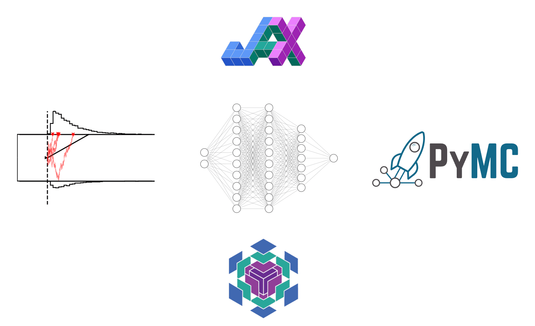
Leaning on an applied data-analysis problem in the cognitive modeling space, this post develops the tools to use neural networks trained with the Flax package (a neural network library based on JAX) as approximate likelihoods in likelihood-free inference scenarios. We will spend some time setting up the data analysis problem first, including the modeling framework used and computational bottlenecks that may arise (however if you don't care about the particulars, feel free to skip this part). Then, step by step, we will develop the tools necessary to go from a simple data simulator without access to a likelihood function to Bayesian Inference with PyMC via a custom distribution.

We will try to keep the code as general as possible, to facilitate other use cases with minimal hassle.

Table of Contents

• Setting the Stage
  • The Data Analysis Problem
    • What kind of Data?
    • The model(s)
    • Motivating likelihood free inference
• From model simulation to PyMC model
  • Simulating Data
  • Turning it into Training Data
  • Building and Training the Network
  • Connecting to PyMC
    • Building a custom distribution
    • Plug the custom distribution into a PyMC model
    • Inference example

Setting the Stage

To motivate the modeling effort expounded upon below, let's start by building the case for a particular class of models, beginning with an (somewhat stylized) original data analysis problem.

Consider a dataset from the NeuroRacer experiment, illustrated below with an adapted figure from the original paper.

The player/subject in this experiment is tasked with steering a racing car along a curvy racetrack, while reacting appropriately to appearing traffic signs under time pressure. Traffic signs are either of the target or no target type, the players' reaction appropriately being a button press or no button press respectively.

In the lingo of cognitive scientists, we may consider this game a Go / NoGo type task (press or withhold depending on traffic sign), under extra cognitive load (steering the car across the racetrack).

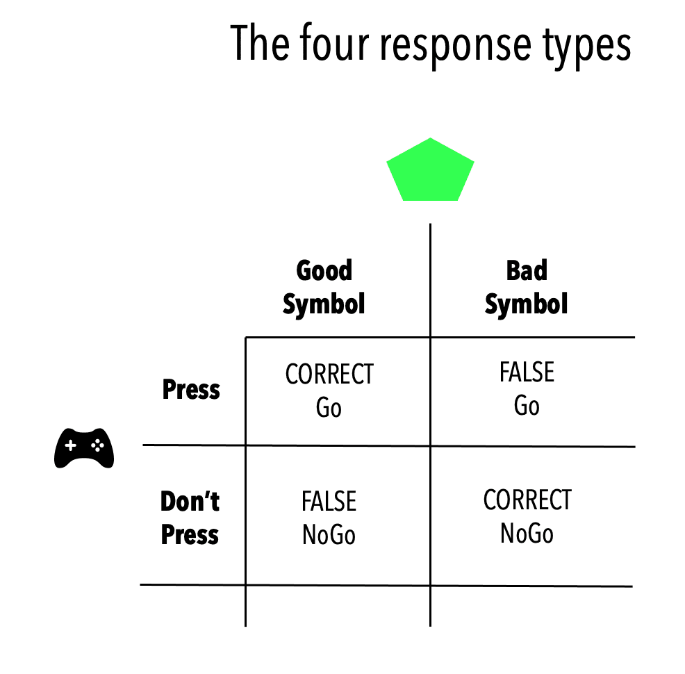
This leaves us with four types of responses to analyse (see the figure below):

1. Correct button press (Correct Go)
2. Correct withhold (Correct NoGo)
3. False button press (False Go)
4. False withhold (False NoGo)

What kind of data

Collecting reaction times (rt) and choices (responses) for each of the trials, our dataset will eventually look as follows.

import numpy as np
import pandas as pd

# Generate example data
data = pd.DataFrame(np.random.uniform(size = (100,1)), columns = ['rt'])
data['response'] = 'go'
data['response'].values[int(data.shape[0] / 2):] = 'nogo'
data['trial_type'] = 'target'
data['trial_type'].values[int(data.shape[0] / 2):] = 'notarget'

data

The model(s)

Cognitive scientists have powerful framework for the joint analysis of reaction time and choice data: Sequential Sampling Models (SSMs).

The canonical model in this framework is the Drift Diffusion Model (or Diffusion Decision Model). We will take this model as a starting point to explain how it applies to the analysis of NeuroRacer data.

The basic idea behind the Drift Diffusion Model is the following. We represent the decision process between two options as a Gaussian random walk of a so-called evidence state. The random walk starts after some non-decision time period following the stimulus appearance. The process then starts at a specific value (parameter ) and evolves according to a deterministic drift (parameter ), perturbed by Gaussian noise. Eventually this process reaches a value that crosses one of two boundaries, which determines the response given by the participant: go or no-go. The distance between the two boundaries is given by a fourth parameter ().

Which bound is reached, and the time of crossing, jointly determine the reaction time and choice. Hence, this model specifies a stochastic data generating process and we can define a likelihood function for this.

However, this likelihood function may be quite hard to derive, and possibly too computationally expensive. As an alternative, we will use a general function approximation via Neural Networks in this tutorial.

Let's first look at an illustration of the model and identify the quantities relevant for our example.

A nice aspect of the Drift Diffusion Model (or Diffusion Decision Model) is that the parameters are interpretationally distinct.

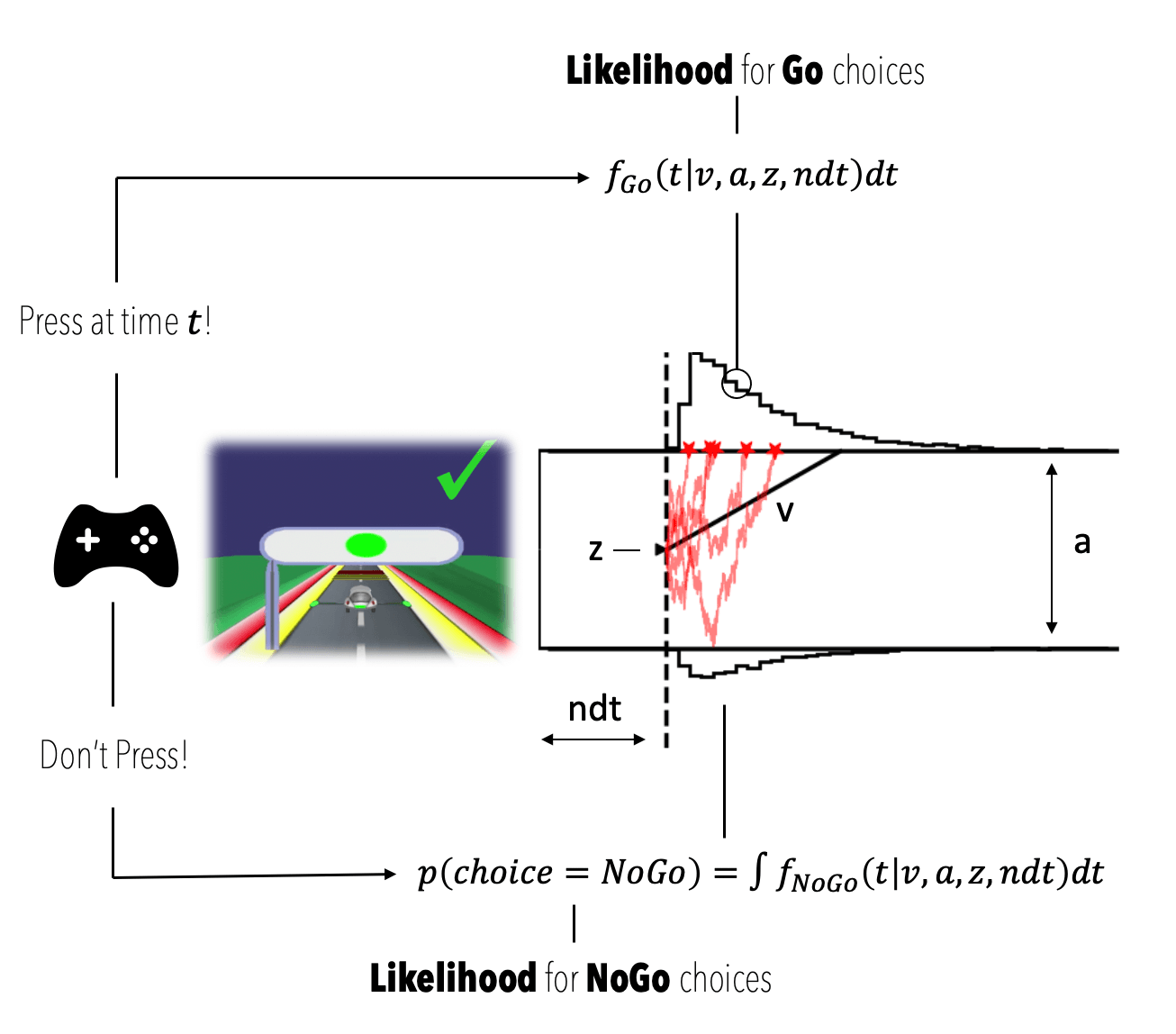
1. , the non-decision time component captures all aspects of decision-time not explicitly modeled as per the random walk process (e.g. motor-preparation, initial time-to-attentive-state etc. etc.)
2. , provides global bias of the process towards one or the other choice. One can think of it as an a priori estimate of the underlying frequency of correct choices as per the experiment design.
3. , is the rate with which evidence is consistently accumulated toward one or the other bound (in favor of one or the other choice). One can think of it as speed of processing.
4. , represent a measure of the desired level of certainty before a decision is committed to. It is also referred to as decision caution.

The two quantities we will make explicit in the analyses are the following are (see also figure above),

1. , the likelihood of observing a Go choice at time
2. , the likelihood of "observing" a withheld button press, defined as the integral of over .

We will focus on a simple analysis case, in which we observe hypothetical data from a single player, who plays the game for trials, of which are Go / target trials (the participant should press the button) and of which are NoGo / no target trials (the participant should not press the button).

We will make a simplifying modeling assumption: the rate of evidence accumulation for a NoGo has the same magnitude as that of Go trials but with a flipped sign, meaning participants are less likely to press a button as time goes by. This allows us to estimate a single parameter.

Hence we get .

Motivating Simulation Based Inference

The Drift Diffusion Model actually has a (cumbersome) analytical likelihood, with specialized algorithms for fast evaluation. There are however many interesting variants for which fast computations are hampered by a lack of closed form solutions (see for example here and here).

Take as one example the model illustrated in the figure below,

Conceptually the only difference is that the decision criterion, described in our simple Drift Diffusion Model above with a single parameter , does now vary with time (as a parametric function). This makes sense if e.g. the decision is supposed to be completed under deadline pressure (in fact this would be the case in our NeuroRacer example). As time progresses, it may be rational to decrease ones decision caution to force an, at least somewhat, informed decision over a guaranteed failure due to missing the deadline (for some reasearch along those lines see for example this paper).

On the other hand simulators for such variants tend to remain easy to code up (often a few lines in python do the job). A simulator but no likelihood? Welcome to the world of simulation based inference (SBI).

Surveying the field of SBI is beyond the scope of this blog post (the paper above is a good start for those interested), but let it be said that SBI is the overarching paradigm from which we pick a specific method to construct our approach below.

The idea is the following. We start with a simulator for the DDM from which, given a set of parameters (, , , ) we can construct empirical likelihood functions for both and . For we construct smoothed histograms (or Kernel Density Estimates), while for we simply collect the respective choice probability from simulation runs.

From these building blocks, we will construct training data to train two Multilayer Perceptrons (MLPs, read: small Neural Networks), one for each of the two parts of the overall likelihood.

These MLPs are going to act as our likelihood functions. We will call the network which represents a LAN, for Likelihood Approximation Network. The network for will be called a CPN, for Choice Probability Network. As we will see later, can then evaluate our data-likelihood via forward passes through the LAN and CPN.

We will then proceed by wrapping these trained networks into a custom PyMC distribution and finally get samples from our posterior of interest via the Blackjax NUTS sampler, completing our walkthrough.

With all these steps ahead, let's get going!

From model simulation to PyMC model

Simulating Data

In favor of a digestible reading experience, we will use a convenience package to simulate data from the DDM model. This package not only allows us to simulate trajectories, but also includes utilities to directly produce data in a format suitable for downstream neural network training (which is our target here). The mechanics behind training data generation are described in this paper.

For some intuition, let's start with simulating and plotting a simple collection of DDM trajectories, setting the parameters as .

from ssms.basic_simulators import simulator

n_trajectories = 1000
parameter_vector = np.array([1.0, 1.5, 0.5, 0.5, 0.5])

simulation_data = simulator(model = 'angle',
                            theta = parameter_vector,
                            n_samples = n_trajectories,
                            random_state = 42)

simulation_data.keys()

dict_keys(['rts', 'choices', 'metadata'])

The simulator returns a dictionary with three keys.

1. rts, the reaction times for each choice under 2.
2. choices, here coded as for lower boundary crossings and for upper boundary crossings.
3. metadata, extra information about the simulator settings

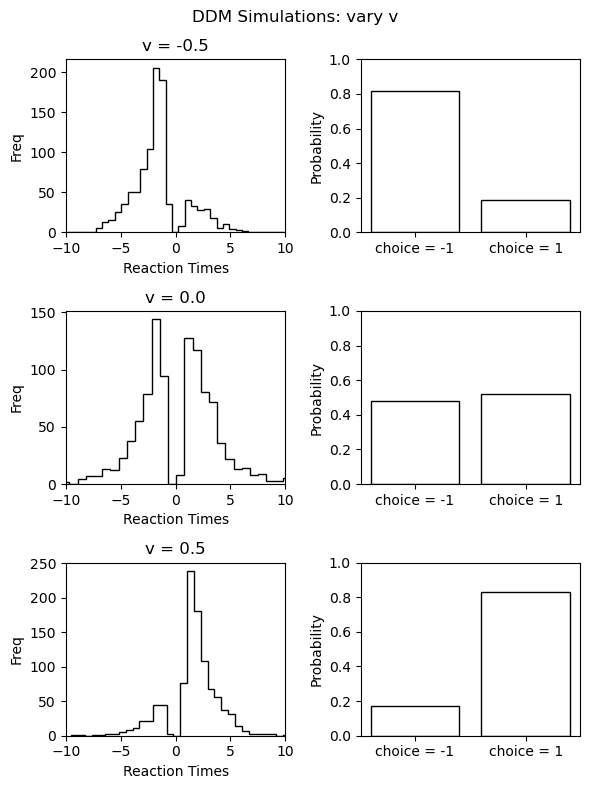
Let's use this to plot the reaction time distribution (negative reals refer to choices) and choice probabilities. We will plot this for a few parameter settings to give some intuition about how the model behaves in response. Specifically we will vary the parameter, holding all other parameters constant the values reported above.

from matplotlib import pyplot as plt
parameter_matrix = np.zeros((3, 4))

# vary the first parameter across rows (the 'v' parameter in our case')
parameter_matrix[:, 0] = np.linspace(-0.5, 0.5, 3)

# set the rest to the values used above
for i in range(1, 4, 1):
    parameter_matrix[:, i] = parameter_vector[i]
    
# Make Figure
fig, axs = plt.subplots(3,2, figsize = (6, 8))
fig.suptitle('DDM Simulations: vary v')
for i in range(3):
    simulation_data_tmp = simulator(model = 'ddm',
                                theta = parameter_matrix[i, :],
                                n_samples = n_trajectories)
    for j in range(2):
        if j == 0:
            # Reaction Times + Choices
            axs[i, j].hist(np.squeeze(simulation_data_tmp['rts']) * np.squeeze(simulation_data_tmp['choices']),
                       histtype = 'step',
                       color = 'black',
                       bins = 40,
                       )
            axs[i, j].set_title('v = ' + str(round(parameter_matrix[i, 0], 2)))
            axs[i, j].set_xlim(-10, 10)
            axs[i, j].set_xlabel('Reaction Times')
            axs[i, j].set_ylabel('Freq')
            axs[i, j]
        else: 
            # Choice probabilities
            p_up = np.sum(simulation_data_tmp['choices'] == 1.) / n_trajectories
            choice_ps = [1 - p_up, p_up]
            axs[i, j].bar(['choice = -1', 'choice = 1'], choice_ps, fill = None)
            axs[i, j].set_ylabel('Probability')
            axs[i, j].set_ylim(0, 1)
fig.tight_layout()
plt.show()

Turning it into Training Data

We will now use a couple of convenience functions from the ssm-simulators package, to generate training data for our Neural Networks. This will proceed in two steps. We first define two config dictionaries to specify properties of the simulation runs that will serve as the basis for our training data set.

1. The generator_config which specifies how to construct training data on top of basic simulations runs.
2. The model_config which specifies the properties of the core simulator.

Second, we will actually run the necessary simulations.

Let's make the config dictionaries.

NOTE:

The details here are quite immaterial. We simply need some way of generating training data of two types.

1. One (for the LAN), which has as features vectors of the kind and as labels corresponding empirical log-likelihood evaluations .

2. One (for the CPN), which takes as features simply the parameter vectors and as labels corresponding empirical choice probabilities .

# MAKE CONFIGS
from ssms.config import data_generator_config
from ssms.config import model_config
from copy import deepcopy

# Generator Config

# (We start from a supplied example in the ssms package)
ddm_generator_config = deepcopy(data_generator_config['lan']) 

# Specify generative model 
# (one from the list of included models in the ssms package / or a single string)
ddm_generator_config['dgp_list'] = 'ddm'

# Specify number of parameter sets to simulate
ddm_generator_config['n_parameter_sets'] = 1000

# Specify how many samples a simulation run should entail
# (To construct an empirical likelihood)
ddm_generator_config['n_samples'] = 10000

# Specify how many training examples to extract from 
# a single parameter vector
ddm_generator_config['n_training_samples_by_parameter_set'] = 2000

# Specify folder in which to save generated data
ddm_generator_config['output_folder'] = 'data/training_data/ddm_high_prec/'

# Model Config
ddm_model_config = model_config['ddm']

We are now in the position to actually run the simulations.

If you run this by yourself,

1. Be aware that the next cell may run for a while (between a few minutes and an hour)
2. Make sure the output_folder specified above exists.

# MAKE DATA
from ssms.dataset_generators import data_generator
n_datasets = 20

# Instantiate a data generator (we pass our configs)
my_dataset_generator = data_generator(generator_config = ddm_generator_config,
                                      model_config = ddm_model_config)

for i in range(n_datasets):
    print('Dataset: ', i + 1, ' of ', n_datasets)
    training_data = my_dataset_generator.generate_data_training_uniform(save = True,
                                                                        verbose = True)

Let's take a quick look at the type of data we generated here (if you run this by yourself, pick one of the unique file names generated during your run):

import pickle
training_data_example = pickle.load(open('data/training_data/ddm_high_prec/training_data_167fc318b85511ed81623ceceff2f96e.pickle', 
                                         'rb'))

training_data_example.keys()

dict_keys(['data', 'labels', 'choice_p', 'thetas', 'binned_128', 'binned_256', 'generator_config', 'model_config'])

Under the data key (this is a legacy name, it might more appropriately called features directly) we find the feature set we need for LANS. A matrix that contains columns [v, a, z, ndt, rt, choice]. In general, across simulator models, the leading columns contain the parameters of the model, the remaining columns contain columns concerning the output data (in our case: responses and choices).

training_data_example['data'][:10, :]

array([[-1.320654 ,  2.4610643,  0.7317903,  1.5463215,  3.5173764,
        -1.       ],
       [-1.320654 ,  2.4610643,  0.7317903,  1.5463215,  5.126489 ,
        -1.       ],
       [-1.320654 ,  2.4610643,  0.7317903,  1.5463215,  4.1766562,
        -1.       ],
       [-1.320654 ,  2.4610643,  0.7317903,  1.5463215,  5.331864 ,
        -1.       ],
       [-1.320654 ,  2.4610643,  0.7317903,  1.5463215,  3.1934366,
        -1.       ],
       [-1.320654 ,  2.4610643,  0.7317903,  1.5463215,  3.8244245,
        -1.       ],
       [-1.320654 ,  2.4610643,  0.7317903,  1.5463215,  5.069471 ,
        -1.       ],
       [-1.320654 ,  2.4610643,  0.7317903,  1.5463215,  6.12916  ,
        -1.       ],
       [-1.320654 ,  2.4610643,  0.7317903,  1.5463215,  4.563048 ,
        -1.       ],
       [-1.320654 ,  2.4610643,  0.7317903,  1.5463215,  4.2055674,
        -1.       ]], dtype=float32)

The labels key, contains the empirical labels.

training_data_example['labels'][:10]

array([-0.9136966 , -1.7495332 , -1.1017948 , -1.9210151 , -1.0180298 ,
       -0.96904343, -1.7043545 , -2.6625948 , -1.3647802 , -1.1204832 ],
      dtype=float32)

The final keys we will be interested in, concern the feature and label data useful for training the CPN networks. This network is a function from the model parameters (theta key) directly to choice probabilities (choice_p key).

training_data_example['thetas'][:10]

array([[-1.320654  ,  2.4610643 ,  0.7317903 ,  1.5463215 ],
       [ 0.6651015 ,  2.032305  ,  0.43455952,  0.39412627],
       [-0.50315803,  2.434122  ,  0.225012  ,  0.9221967 ],
       [-0.2956373 ,  1.1780746 ,  0.3984416 ,  1.361724  ],
       [-0.39936534,  1.170804  ,  0.57806057,  1.2206811 ],
       [-1.1943408 ,  0.68256736,  0.6976298 ,  1.172115  ],
       [ 0.7937759 ,  2.049422  ,  0.45930618,  0.48710603],
       [-2.0405245 ,  2.453905  ,  0.7521208 ,  1.9120167 ],
       [-2.8156106 ,  2.2226427 ,  0.69219965,  1.0444195 ],
       [ 0.37362418,  1.775074  ,  0.42867982,  0.22735284]],
      dtype=float32)

training_data_example['choice_p'][:10]

array([2.930e-02, 9.146e-01, 1.540e-02, 2.471e-01, 3.542e-01, 3.422e-01,
       9.555e-01, 6.300e-03, 7.000e-04, 7.356e-01], dtype=float32)

There are a few other keys in the training_data_example dictionary. We can ignore these for the purposes of this blog post.

We are ready to move forward by turning our raw training data into a DataLoader object, which directly prepares for ingestion by the Neural Networks.

The DataLoader is supposed take care of:

1. Efficiently reading in datafiles and
2. turning them into batches to be ingested when training a Neural Network.

As has become somewhat of a standard, will work off of the Dataset class supplied by the torch.utils.data module in the PyTorch deep learning framework.

The key methods to define in our custom dataset are __getitem__() and __len__().

__len__() helps us to understand the amount of batches contained in a complete run through the data (epoch in machine learning lingo). __getitem_() is the method called to retrieve the next batch of data.

Let's construct it.

import torch
from __future__ import annotations
from typing import List
from typing import Type

class DatasetTorch(torch.utils.data.Dataset):
    def __init__(self,
                 file_ids: List[str] | None = None,
                 batch_size: int = 32,
                 label_lower_bound: float | None = None,
                 features_key: str = 'data',
                 label_key: str = 'labels',
                 ) -> Type[torch.utils.dataDataset]:
        
        # Initialization
        self.batch_size = batch_size
        self.file_ids = file_ids
        self.indexes = np.arange(len(self.file_ids))
        self.label_lower_bound = label_lower_bound
        self.features_key = features_key
        self.label_key = label_key
        self.tmp_data = None

        # Get metadata from loading a test file
        self.__init_file_shape()

    def __len__(self):
        """
        Calculates number of batches per epoch.
        """
        return int(np.floor((len(self.file_ids) * ((self.file_shape_dict['inputs'][0] // self.batch_size) * self.batch_size)) / self.batch_size))

    def __getitem__(self, index: int):
        """
        Return next batch.
        """
        # Check if it is time to load the next file from disk
        if index % self.batches_per_file == 0 or self.tmp_data == None:
            self.__load_file(file_index = self.indexes[index // self.batches_per_file])

        # Generate batch_ids
        batch_ids = np.arange(((index % self.batches_per_file) * self.batch_size), 
                              ((index % self.batches_per_file) + 1) * self.batch_size, 1)
        
        # Make corresponding batch
        X = self.tmp_data[self.features_key][batch_ids, :]
        y = np.expand_dims(self.tmp_data[self.label_key][batch_ids], axis = 1)
        
        # Apply lower bound on labels
        if self.label_lower_bound is not None:
            y[y < self.label_lower_bound] = self.label_lower_bound 
        return X, y

    def __load_file(self, file_index: int):
        """
        Load new file if requested.
        """
        # Load file and shuffle the indices
        self.tmp_data = pickle.load(open(self.file_ids[file_index], 'rb'))
        shuffle_idx = np.random.choice(self.tmp_data[self.features_key].shape[0], 
                                        size = self.tmp_data[self.features_key].shape[0],
                                         replace = True)
        self.tmp_data[self.features_key] = self.tmp_data[self.features_key][shuffle_idx, :]
        self.tmp_data[self.label_key] = self.tmp_data[self.label_key][shuffle_idx]
        return

    def __init_file_shape(self):
        """
        Set data shapes during initialization.
        """
        # Function gets dimensionalities form a test data file 
        # (first in the supplied list of file names)
        init_file = pickle.load(open(self.file_ids[0], 'rb'))
        self.file_shape_dict = {'inputs': init_file[self.features_key].shape, 
                                'labels': init_file[self.label_key].shape}
        self.batches_per_file = int(self.file_shape_dict['inputs'][0] / self.batch_size)
        self.input_dim = self.file_shape_dict['inputs'][1]

        if len(self.file_shape_dict['labels']) > 1:
            self.label_dim = self.file_shape_dict['labels'][1]
        else:
            self.label_dim = 1
        return

Let's construct our training dataloaders for both our LAN and CPN networks (which we will define next). We use the DataLoader class in the torch.utils.data module to turn our Dataset class into an iterator.

NOTE:

To not explode code blocks in this blog post, we will only concern ourselves with training data here, instead of including (as one should in a serious machine learning application) DataLoader classes for validation data as well. Defining validation data works analogously.

Notice how we change the features_key and label_key arguments to access the relevant part of our training data files respectively for the LAN and CPN.

import os 
import pickle

# MAKE DATALOADERS

# List of datafiles (here only one)
folder_ = 'data/training_data/ddm_high_prec/'
file_list_ = [folder_ + file_ for file_ in os.listdir(folder_) if '.ipynb' not in file_]

# Training datasets
training_dataset_lan = DatasetTorch(file_ids = file_list_,
                                    batch_size = 8192,
                                    label_lower_bound = np.log(1e-7),
                                    features_key = 'data',
                                    label_key = 'labels',
                                    )

training_dataset_cpn = DatasetTorch(file_ids = file_list_,
                                    batch_size = 512,
                                    features_key = 'thetas',
                                    label_key = 'choice_p',
                                    )

# Training dataloaders
training_dataloader_lan = torch.utils.data.DataLoader(training_dataset_lan,
                                                      shuffle = True,
                                                      batch_size = None,
                                                      num_workers = 1,
                                                      pin_memory = True
                                                     )

training_dataloader_cpn = torch.utils.data.DataLoader(training_dataset_cpn,
                                                      shuffle = True,
                                                      batch_size = None,
                                                      num_workers = 1,
                                                      pin_memory = True
                                                     )

Building and Training the Network

We used the simulator to construct training data and constructed dataloaders on top of that. It is time to build and train our networks!

We will use the Flax python package for this purpose. Let's first define a basic neural network class, constrained to minimal functionality. We build such a class by inheriting from the nn.Module class in the flax.linen module and specifying two methods.

1. The setup() method, which will be run as a preparatory step upon instantiation.
2. The __call__() metod defines the forward pass through the network.

from flax import linen as nn
from frozendict import frozendict
from typing import Sequence

class MLPJax(nn.Module):
    """
    Basic Neural Network class as per the Flax package for neural network 
    modeling with Jax.
    """
    layer_sizes: Sequence[int] = (100, 100, 100, 1)
    activations: Sequence[str] = ('tanh', 'tanh', 'tanh', 'linear')
    train: bool = True # if train = False, output applies transform f such that: f(train_output_type) = logprob
    train_output_type: str = 'logprob'
    activations_dict = frozendict({'relu': nn.relu,
                                   'tanh': nn.tanh,
                                   'sigmoid': nn.sigmoid
                                  })
        
    def setup(self):
        # Assign layers and activation functions as class attributes
        self.layers = [nn.Dense(layer_size) for layer_size in self.layer_sizes]
        self.activation_funs = [self.activations_dict[activation] for \
                                activation in self.activations if (activation != 'linear')]
    
    def __call__(self, inputs: Type[jax.numpy.array]) -> Type[jax.numpy.array]:
        """
        This is used to define the forward pass, which will later be called via
        mymodel.apply(state, input)
        """
        
        # Define forward pass
        x = inputs
        
        # Cycle through layers
        for i, lyr in enumerate(self.layers):
            x = lyr(x)
            if i != (len(self.layers) - 1):
                x = self.activation_funs[i](x)
            else:
                if self.activations[i] == 'linear': 
                    pass
                else:
                    x = self.activation_funs[i](x)
        
        # Apply potential transform of outputs if in eval model
        if not self.train and self.train_output_type == 'logits':
            return - jax.numpy.log((1 + jax.numpy.exp(-x)))
        else:
            return x
    
    def make_forward_partial(self,
                             state = None,
                            ):
        """
        Make a single-argument forward pass function (only network input needed instead
        of needing to pass the network state as well).
        """

        net_forward = partial(self.apply, state)
        net_forward_jitted = jax.jit(net_forward)

        return net_forward, net_forward_jitted

Next we define a Neural Network trainer class. This will take a MLPJax instance and build the necessary infrastructure for network training around it. The approach roughly follows the suggestions in the Flax documentation.

import jax
import optax
from optax import warmup_cosine_decay_schedule
from optax import huber_loss
from optax import sigmoid_binary_cross_entropy
from optax import l2_loss

from flax.training import train_state
from functools import partial

from tqdm import tqdm

class ModelTrainerJaxMLP:
    def __init__(self,
                 model: Type[nn.Module] = None,
                 loss: Dict[str, Any] | str | None = None,
                 train_dl: Type[torch.utils.data.DataLoader] | None = None,
                 seed: int | None = None):
        
        # Provide some options for loss functions
        self.loss_dict = {'huber': {'fun': huber_loss,
                               'kwargs': {'delta': 1}},
                          'mse': {'fun': l2_loss,
                                 'kwargs': {}},
                          'bcelogit': {'fun': sigmoid_binary_cross_entropy,
                                      'kwargs': {}}
                         }
        
        self.model = model
        self.train_dl = train_dl
        self.loss = loss
        self.dataset_len = self.train_dl.dataset.__len__()
        self.seed = seed
        
        self.__get_loss()
        self.apply_model = self.__make_apply_model()
        self.update_model = self.__make_update_model()
            
    def __get_loss(self):
        self.loss = partial(self.loss_dict[self.loss]['fun'], 
                            **self.loss_dict[self.loss]['kwargs'])
    
    def __make_apply_model(self):
        """
        Construct jitted forward and backward pass.
        """
        @jax.jit
        def apply_model_core(state, features, labels):
            def loss_fn(params):
                pred = state.apply_fn(params, features)
                loss = jax.numpy.mean(self.loss(pred, labels))
                return loss, pred
            
            grad_fn = jax.value_and_grad(loss_fn, has_aux = True)
            (loss, pred), grads = grad_fn(state.params)
            return grads, loss
        
        return apply_model_core
    
    def __make_update_model(self):
        """
        Construct jitted optimizer step
        """
        @jax.jit
        def update_model(state, grads):
            return state.apply_gradients(grads = grads)
        return update_model
        
    def create_train_state(self, rng: int, n_epochs: int):
        """
        Create a TrainState object that is essentially a convenience object for 
        storing a given networks' foward pass, parameter state, and optimizer state.
        """
        params = self.model.init(rng, jax.numpy.ones((1, self.train_dl.dataset.input_dim)))
        lr_schedule = warmup_cosine_decay_schedule(init_value = 0.0002,
                                                   peak_value = 0.02,
                                                   warmup_steps = self.dataset_len,
                                                   decay_steps = self.dataset_len * \
                                                                 n_epochs,
                                                   end_value = 0.0)
        tx = optax.adam(learning_rate = lr_schedule)
        return train_state.TrainState.create(apply_fn = self.model.apply,
                                             params = params,
                                             tx = tx)
    
    def run_epoch(self,
                  state,
                  train: bool = True):
        """
        Run single epoch
        """
        
        epoch_loss = []
        for X, y in tqdm(self.train_dl):
            X_jax = jax.numpy.array(X)
            y_jax = jax.numpy.array(y)
            
            grads, loss = self.apply_model(state, X_jax, y_jax)
            state = self.update_model(state, grads)
            epoch_loss.append(loss)
                    
        mean_epoch_loss = np.mean(epoch_loss)
        return state, mean_epoch_loss
    
    def train(self,
              n_epochs: int = 25):
        """
        Train the network for the chosen number of epochs.
        """
        
        # Initialize network
        rng = jax.random.PRNGKey(self.seed)
        rng, init_rng = jax.random.split(rng)
        state = self.create_train_state(init_rng,
                                        n_epochs = n_epochs)

        # Training loop over epochs
        for epoch in range(n_epochs):
            state, train_loss = self.run_epoch(state, train = True)
            print('Epoch: {} / {}, test_loss: {}'.format(epoch, n_epochs, 
                                                         train_loss))

        self.state = state
        return state

Preparations are all you need! We can now train our LAN and CPN with a few lines of code, making use of our previously defined classes.

# Initialize LAN
network_lan = MLPJax(train = True, # if train = False, output applies transform f such that: f(train_output_type) = logprob
                     train_output_type = 'logprob')

# Set up the model trainer                                
ModelTrainerLAN = ModelTrainerJaxMLP(model = network_lan,
                                     train_dl = training_dataloader_lan,
                                     loss = 'huber',
                                     seed = 123)

# Train LAN
model_state_lan = ModelTrainerLAN.train(n_epochs = 10)

100%|██████████| 4880/4880 [00:30<00:00, 159.70it/s]


Epoch: 1 / 10, test_loss: 0.14862245321273804


 ...


100%|██████████| 4880/4880 [00:28<00:00, 169.85it/s]


Epoch: 10 / 10, test_loss: 0.01756889559328556

# Initialize CPN
network_cpn = MLPJax(train = True,
                     train_output_type = 'logits')

# Set up the model trainer                                
ModelTrainerCPN = ModelTrainerJaxMLP(model = network_cpn,
                                     train_dl = training_dataloader_cpn,
                                     loss = 'bcelogit',
                                     seed = 456)

# Train CPN
model_state_cpn = ModelTrainerCPN.train(n_epochs = 20)

100%|██████████| 20/20 [00:02<00:00,  9.14it/s]


Epoch: 1 / 20, test_loss: 0.42765116691589355


...


100%|██████████| 20/20 [00:00<00:00, 27.14it/s]

Epoch: 20 / 20, test_loss: 0.30409830808639526

Connecting to PyMC

At this point we have two networks ready (we will later see example output that illustrate the behavior / quality of the approximation), which can be used as differentiable approximations to likelihood evaluations. The figure below should illustrate the respective function of each network (e.g. in the Go condition). This may help as a guiding visualization for the subsequent content.

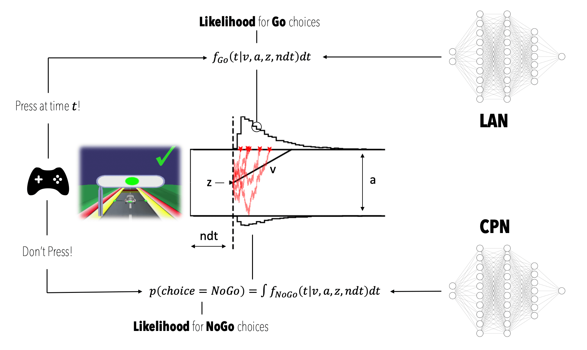
A CPN, which we will use as an approximator to,

and,

A LAN, which we will use as an approximator to,

where refers to the log-likelihood.

Together the CPN and the LAN allow us to construct a likelihood for a complete dataset from the NeuroRacer game.

Take the complete likelihood for a dataset of size , for trials in which the traffic sign warrants a button press (Go Condition). We can split our dataset into two parts.

1. Go condition, Go choice (we observe a reaction time):
2. Go condition, NoGo choice (we don't observe a reaction time):

The log likelihood of the Go condition data can now be represented as:

For the NoGo Condition, we essentially apply the same logic so that the log likelihood of the NoGo condition data can now be represented as:

As per our modeling assumption we switch set , to get the full data log-likelihood,

Building a custom distribution

All pieces are lined up to start building a custom distribution for eventual use in a PyMC model. The starting point has to be the construction of a custom likelihood, as a valid PyTensor Op. For this purpose we use the NetworkLike class below. It allows us to construct proper log-likelihoods from our two networks.

What do we mean by proper log-likelihood?

A valid Jax function that takes in parameters, processes the input data, performs the appropriate forward pass through the networks, and finally sums the resulting trial-wise log-likelihoods to give us a data-log-likelihood. This is taken care of by the make_logp_jax_funcs() method.

Finally we need to turn these isolated likelihood functions into a valid PyTensor Op, which is taken care of by the make_jax_logp_ops() function. Note how we also register our log-likelihood function directly as a Jax log-likelihood (unwrap it) using the jax.funcify decorator with the logp_op_dispatch() method. This log-likelihood function does not need to be compiled (note how we pass the logp_nojit likelihood there), which will instead be taken care of by any of the Jax sampler that PyMC provides (via NumPyro, or BlackJax)

NOTE:

The below code is a little involved and could be hard to digest on a first pass. Consider looking into the excellent tutorials in the PyMC docs and the PyMC Labs Blog on similar topics.

Specifically, the tutorial on using a blackbox likelihood function, the tutorial on custom distributions, the tutorial on wrapping jax functions into PyTensor Ops.

Finally there is an excellent tutorial from PyMC Labs, which incorporates Flax to train Bayesian Neural Networks (amongst other things): A different spin on our story here, not exactly equivalent, but helpful to understand the scope of use-cases encompassed at the intersection of Neural Networks and the Bayesian workflow.

from os import PathLike
from typing import Callable, Tuple

import pytensor 
pytensor.config.floatX = "float32"
import pytensor.tensor as pt
import jax.numpy as jnp
import numpy as np
from pytensor.graph import Apply, Op
from pytensor.link.jax.dispatch import jax_funcify
from jax import grad, jit
from numpy.typing import ArrayLike

LogLikeFunc = Callable[..., ArrayLike]
LogLikeGrad = Callable[..., ArrayLike]

import pymc as pm
from pytensor.tensor.random.op import RandomVariable

import warnings 
warnings.filterwarnings('ignore')

class NetworkLike:
    @classmethod
    def make_logp_jax_funcs(
        cls,
        model = None,
        n_params: int | None = None,
        kind: str = 'lan',
    ) -> Tuple[LogLikeFunc, LogLikeGrad, LogLikeFunc,]:
        """Makes a jax log likelihood function from flax network forward pass.
        Args:
            model: A path or url to the ONNX model, or an ONNX Model object
            already loaded.
            compile: Whether to use jit in jax to compile the model.
        Returns: A triple of jax or Python functions. The first calculates the
            forward pass, the second calculates the gradient, and the third is
            the forward-pass that's not jitted.
        """
        if kind == 'lan':
            def logp_lan(data: np.ndarray, *dist_params) -> ArrayLike:
                """
                Computes the sum of the log-likelihoods given data and arbitrary
                numbers of parameters assuming the trial by trial likelihoods
                are derived from a LAN.
                Args:
                    data: response time with sign indicating direction.
                    dist_params: a list of parameters used in the likelihood computation.
                Returns:
                    The sum of log-likelihoods.
                """

                # Makes a matrix to feed to the LAN model
                params_matrix = jnp.repeat(
                    jnp.stack(dist_params).reshape(1, -1), axis=0, repeats=data.shape[0]
                )

                # Set 'v' parameters depending on condition
                params_matrix = params_matrix.at[:, 0].set(params_matrix[:, 0] * data[:, 2])

                # Stack parameters and data to have full input
                input_matrix = jnp.hstack([params_matrix, data[:, :2]])

                # Network forward and sum
                return jnp.sum(
                    jnp.squeeze(model(input_matrix))
                )
            
            logp_grad_lan = grad(logp_lan, argnums=range(1, 1 + n_params))
            return jit(logp_lan), jit(logp_grad_lan), logp_lan
            
        elif kind == 'cpn':
            def logp_cpn(data: np.ndarray, *dist_params) -> ArrayLike:
                """
                Computes the sum of the log-likelihoods given data and arbitrary
                numbers of parameters assuming the trial-by-trial likelihood derive for a CPN.
                Args:
                    data: response time with sign indicating direction.
                    dist_params: a list of parameters used in the likelihood computation.
                Returns:
                    The sum of log-likelihoods.
                """

                # Makes a matrix to feed to the LAN model
                n_nogo_go_condition = jnp.sum(data > 0)
                n_nogo_nogo_condition = jnp.sum(data < 0)
                dist_params_go  = jnp.stack(dist_params).reshape(1, -1)

                # AF-TODO Bugfix here !
                dist_params_nogo = jnp.stack(dist_params).reshape(1, -1)
                dist_params_nogo = dist_params_nogo.at[0].set((-1) * dist_params_nogo[0])

                net_in = jnp.vstack([dist_params_go, dist_params_nogo])

                net_out = jnp.squeeze(model(net_in))

                out = (jnp.log(1 - jnp.exp(net_out[0])) * n_nogo_go_condition) + \
                        (jnp.log(1 - jnp.exp(net_out[1])) * n_nogo_nogo_condition)

                return out

            logp_grad_cpn = grad(logp_cpn, argnums=range(1, 1 + n_params))
            return jit(logp_cpn), jit(logp_grad_cpn), logp_cpn
    
    @staticmethod
    def make_jax_logp_ops(
        logp: LogLikeFunc,
        logp_grad: LogLikeGrad,
        logp_nojit: LogLikeFunc,
    ) -> LogLikeFunc:
        """Wraps the JAX functions and its gradient in Pytensor Ops.
        Args:
            logp: A JAX function that represents the feed-forward operation of the
                LAN network.
            logp_grad: The derivative of the above function.
            logp_nojit: A Jax function
        Returns:
            An pytensor op that wraps the feed-forward operation and can be used with
            pytensor.grad.
        """

        class LogpOp(Op):
            """Wraps a JAX function in an pytensor Op."""

            def make_node(self, data, *dist_params):
                inputs = [
                    pt.as_tensor_variable(data),
                ] + [pt.as_tensor_variable(dist_param) for dist_param in dist_params]

                outputs = [pt.scalar()]

                return Apply(self, inputs, outputs)

            def perform(self, node, inputs, output_storage):
                """Performs the Apply node.
                Args:
                    inputs: This is a list of data from which the values stored in
                        output_storage are to be computed using non-symbolic language.
                    output_storage: This is a list of storage cells where the output
                        is to be stored. A storage cell is a one-element list. It is
                        forbidden to change the length of the list(s) contained in
                        output_storage. There is one storage cell for each output of
                        the Op.
                """
                result = logp(*inputs)
                output_storage[0][0] = np.asarray(result, dtype=node.outputs[0].dtype)

            def grad(self, inputs, output_grads):
                results = lan_logp_grad_op(*inputs)
                output_gradient = output_grads[0]
                return [
                    pytensor.gradient.grad_not_implemented(self, 0, inputs[0]),
                ] + [output_gradient * result for result in results]

        class LogpGradOp(Op):
            """Wraps the gradient opearation of a jax function in an pytensor op."""

            def make_node(self, data, *dist_params):
                inputs = [
                    pt.as_tensor_variable(data),
                ] + [pt.as_tensor_variable(dist_param) for dist_param in dist_params]
                outputs = [inp.type() for inp in inputs[1:]]

                return Apply(self, inputs, outputs)

            def perform(self, node, inputs, outputs):
                results = logp_grad(inputs[0], *inputs[1:])

                for i, result in enumerate(results):
                    outputs[i][0] = np.asarray(result, dtype=node.outputs[i].dtype)

        lan_logp_op = LogpOp()
        lan_logp_grad_op = LogpGradOp()

        # Unwraps the JAX function for sampling with JAX backend.
        @jax_funcify.register(LogpOp) # Can fail in notebooks
        def logp_op_dispatch(op, **kwargs):  # pylint: disable=W0612,W0613
            return logp_nojit

        return lan_logp_op

The likelihood class will come in handy when defining our PyMC model below .

We now construct simple forward functions for our networks (lan_forward(), cpn_forward()). We use the make_forward_partial() method of our previously defined MLPJax class.

First we instantiate the networks in evaluation mode. The make_forward_partial() function then attaches our trained parameters to the usual Flax forward call (which takes in two arguments, the parameters and the model input) so that we can call lan_forward() and cpn_forward() with a single argument, the input data to be pushed through the respective network.

As you can check above, the work is done by the partial() function.

# Initialize LAN in evaluation mode
network_lan_eval = MLPJax(train = False,
                          train_output_type = 'logprob')

# Make jitted forward passes (with fixed weights)
lan_forward, _ = network_lan_eval.make_forward_partial(state = ModelTrainerLAN.state.params)


# Initialize CPN in evaluation mode
network_cpn_eval = MLPJax(train = False,
                          train_output_type = 'logits')


# Make jitted forward passes (with fixed weights)
cpn_forward, _ = network_cpn_eval.make_forward_partial(state = ModelTrainerCPN.state.params)                     

As a quick aside, to illustrate the performance of the Networks, we plot their behavior below.

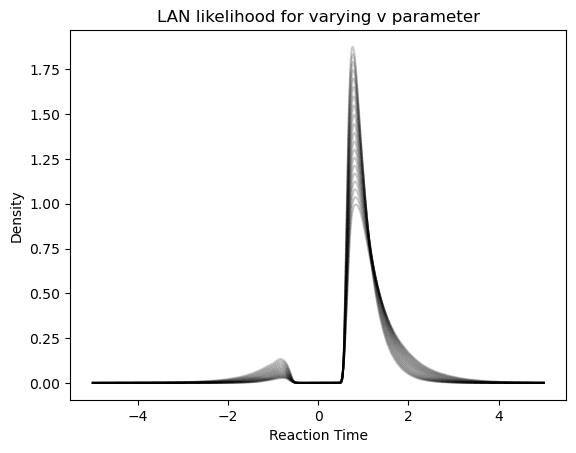
First, consider the LAN, which gives us choice / reaction time distributions directly. We will vary the parameter to illustrate how the likelihood produced by the network varies in response.

# Loop over parameter configurations to plot
# multiple LAN outputs
for i in np.linspace(1., 2., 20):
    inp_ = np.zeros((2000, 6))
    inp_[:, 0] = i # v parameter --> varies
    inp_[:, 1] = 1.0 # a parameter
    inp_[:, 2] = 0.5 # z parameter
    inp_[:, 3] = 0.5 # ndt parameter
    inp_[:, 4] = np.concatenate([np.linspace(5, 0, 1000),
                                 np.linspace(0, 5, 1000)]) # rt
    inp_[:, 5] = np.concatenate([(-1)*np.ones(1000), np.ones(1000)]) # choices


    plt.plot(inp_[:, 4] * inp_[:, 5], jnp.exp(lan_forward(inp_)), color = 'black', alpha = 0.2)
    plt.title('LAN likelihood for varying v parameter')
    plt.xlabel('Reaction Time')
    plt.ylabel('Density')

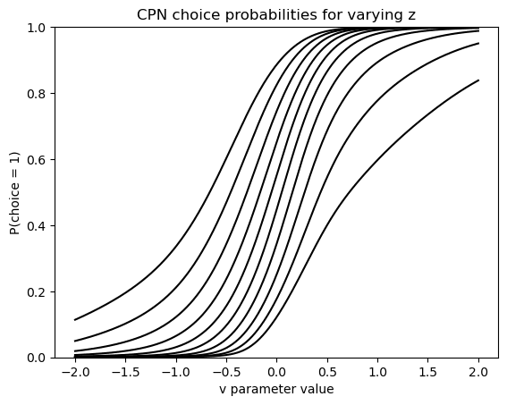
Next we consider the performance of the CPN which, remember, spits out choice probabilities only. In this plot we vary the parameter on the x-axis, and show how the choice probabilities produced by the network vary in reponse. This is repeated for multiple levels of the (or bias) parameter.

# Vary z in outer loop
for i in np.linspace(0.1, 0.9, 10):
    dat_tmp = np.zeros((1000, 4))
    dat_tmp[:, 0] = np.linspace(-2, 2, 1000) # vary v parameter
    dat_tmp[:, 1] = 2.0 # a
    dat_tmp[:, 2] = i # z
    dat_tmp[:, 3] = 1. # ndt / t
    plt.plot(dat_tmp[:, 0], jnp.exp(cpn_forward(dat_tmp)), color = 'black')
    
plt.ylim(0, 1)
plt.title('CPN choice probabilities for varying z')
plt.xlabel('v parameter value')
plt.ylabel('P(choice = 1)')

The outputs of the networks behave very regularly which is reassuring. To see if they match the real data generation process well, let's consider our previous figure on simulator behavior.

parameter_matrix = np.zeros((3, 4))

# vary the first parameter across rows (the 'v' parameter in our case')
parameter_matrix[:, 0] = np.linspace(-0.5, 0.5, 3)

# set the rest to the values used above
for i in range(1, 4, 1):
    parameter_matrix[:, i] = parameter_vector[i]
    
# Make Figure
fig, axs = plt.subplots(3,2, figsize = (6, 8))
fig.suptitle('DDM Simulations: vary v')
for i in range(3):
    simulation_data_tmp = simulator(model = 'ddm',
                                theta = parameter_matrix[i, :],
                                n_samples = n_trajectories)
    
    # LAN
    inp_ = np.zeros((2000, 6))
    inp_[:, 0] = parameter_matrix[i, 0]  # v parameter --> varies
    inp_[:, 1] = parameter_matrix[i, 1], # a parameter
    inp_[:, 2] = parameter_matrix[i, 2], # z parameter
    inp_[:, 3] = parameter_matrix[i, 3], # ndt parameter
    inp_[:, 4] = np.concatenate([np.linspace(5, 0, 1000),
                                 np.linspace(0, 5, 1000)]) # rt
    inp_[:, 5] = np.concatenate([(-1)*np.ones(1000), np.ones(1000)]) # choices
    
    for j in range(2):
        if j == 0:
            # Reaction Times + Choices
            # Simulator
            axs[i, j].hist(np.squeeze(simulation_data_tmp['rts']) * np.squeeze(simulation_data_tmp['choices']),
                       histtype = 'step',
                       color = 'black',
                       bins = 40,
                       density = True,
                       )
            
            # LAN
            axs[i, j].plot(inp_[:, 4] * inp_[:, 5], jnp.exp(lan_forward(inp_)), 
                           color = 'blue', alpha = 0.5)

            axs[i, j].set_title('v = ' + str(round(parameter_matrix[i, 0], 2)))
            axs[i, j].set_xlim(-10, 10)
            axs[i, j].set_xlabel('Reaction Times')
            axs[i, j].set_ylabel('Freq')
            

        else: 
            # Choice probabilities
            p_up = np.sum(simulation_data_tmp['choices'] == 1.) / n_trajectories
            choice_ps = [1 - p_up, p_up]
            
            # Simulator
            axs[i, j].bar(['choice = -1', 'choice = 1'], choice_ps, fill = None)
            
            # CPN
            axs[i, j].scatter(['choice = -1', 'choice = 1'], 
                              [(1 - jnp.exp(cpn_forward(parameter_matrix[i, :]))), 
                               jnp.exp(cpn_forward(parameter_matrix[i, :]))],
                              color = 'blue', alpha = 0.5)
            
            axs[i, j].set_ylabel('Probability')
            axs[i, j].set_ylim(0, 1)
            
fig.tight_layout()
plt.show()

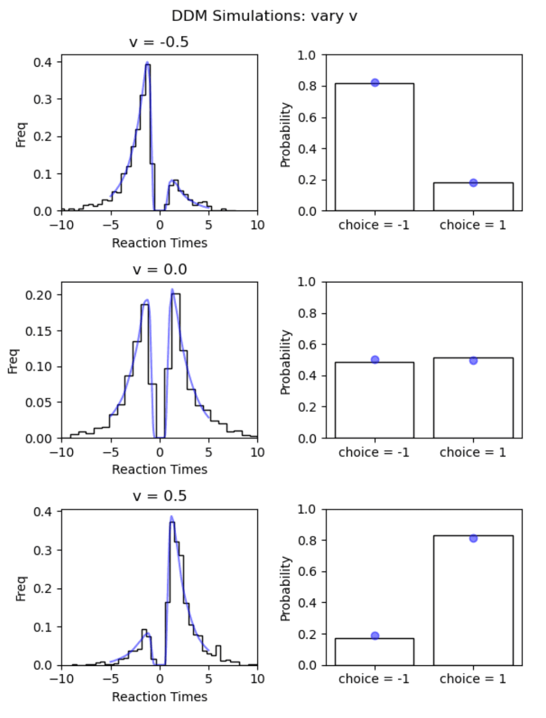
As we can see, the network outputs (shown in blue ) follow the simulation data very well.

NOTE:

We emphasize that for serious applications we are better served using a much larger training data set. The scale of the simulation run here was chosen to make running the code in this blog-post feasible on local machines in a reasonable amount of time.

Plug the custom likelihoods into a PyMC model

Now the hard work in the previous section culminates into actual results. We are able to construct our PyMC model by assembling the pieces we built in the previous sections. We instantiate our LAN and CPN based likelihood ops using the methods defined in our NetworkLike class. First, we define simple like likelihood functions via the make_logp_jax_funcs() method, then we construct the actual PyTensor LogOp's, which will be used directly in the PyMC model below.

# Instantiate LAN logp functions
lan_logp_jitted, lan_logp_grad_jitted, lan_logp = NetworkLike.make_logp_jax_funcs(
                                                                                                 model = lan_forward,
                                                                                                 n_params = 4,
                                                                                                 kind = "lan")

# Turn into logp op
lan_logp_op = NetworkLike.make_jax_logp_ops(
                                logp = lan_logp_jitted,
                                logp_grad = lan_logp_grad_jitted,
                                logp_nojit = lan_logp)

# Instantiate CPN logp functions
cpn_logp_jitted, cpn_logp_grad_jitted, cpn_logp = NetworkLike.make_logp_jax_funcs(
                                                                                                    model = cpn_forward,
                                                                                                    n_params = 4,
                                                                                                    kind = "cpn")

# Turn into logp op
cpn_logp_op = NetworkLike.make_jax_logp_ops(
                                logp = cpn_logp_jitted,
                                logp_grad = cpn_logp_grad_jitted,
                                logp_nojit = cpn_logp)

Finally, let's define a function that constructs our PyMC model for us. Note how we use our likelihood ops, the lan_logp_op() and the cpn_logp_op() respectively to define two pm.Potential() functions. You can learn more about pm.Potential() in the docs, and more connected to blackbox likelihoods, in this helpful basic tutorial.

def construct_pymc_model(data: Type[pd.DataFrame] | None = None):
    """
    Construct our PyMC model given a dataset.
    """
    
    # Data preprocessing:
    # We expect three columns [rt, choice, condition(go or nogo)]
    # We split the data according to whether the choice is go or nogo
    data_nogo = data.loc[data.choice < 0, :]['is_go_trial'].values
    data_go = data.loc[data.choice > 0, :].values
    
    with pm.Model() as ddm:
        # Define simple Uniform priors
        v = pm.Uniform("v", -3.0, 3.0)
        a = pm.Uniform("a", 0.3, 2.5)
        z = pt.constant(0.5)
        t = pm.Uniform("t", 0.0, 2.0)
        
        pm.Potential("choice_rt", lan_logp_op(data_go, v, a, z, t))
        pm.Potential("choice_only", cpn_logp_op(data_nogo, v, a, z, t))
        
    return ddm

Inference example

We are nearing the end of this blog-post (promised). All that remains is to simply try it out. At this point we can simulate some synthetic Neuroracer experiment data, fire up our newly designed PyMC model and run our MCMC sampler for parameter inference.

We pick a set of parameters, and following our modeling assumptions, we apply for the trials we assign to the NoGo condition.

# Let's make some data 
from ssms.basic_simulators import simulator
parameters = {'v': 1.0,
              'a': 1.5,
              'z': 0.5,
              't': 0.5}

parameters_go = [parameters[key_] for key_ in parameters.keys()]
parameters_nogo = [parameters[key_] if key_ != 'v' else ((-1)*parameters[key_]) for key_ in parameters.keys()]

# Run simulations for each condition (go, nogo)
sim_go = simulator(theta = parameters_go, model = 'ddm', n_samples = 500) 
sim_nogo = simulator(theta = parameters_nogo, model = 'ddm', n_samples = 500)

# Process data and add a column that signifies whether the trial,
# belongs to a go (1) or nogo (-1) condition
data_go_condition = np.hstack([sim_go['rts'], sim_go['choices'], np.ones((500, 1))])
data_nogo_condition = np.hstack([sim_nogo['rts'], sim_nogo['choices'], (-1)*np.ones((500, 1))])

# Stack the two datasets and turn into DataFrame
data = np.vstack([data_go_condition, data_nogo_condition]).astype(np.float32)
data_pd = pd.DataFrame(data, columns = ['rt', 'choice', 'is_go_trial'])

Our dataset at hand, we can now intiate the PyMC model.

ddm_blog = construct_pymc_model(data_pd)

Let's visualize the model structure.

pm.model_to_graphviz(ddm_blog)

The graphical model nicely illustrates how we handle the Go choices and NoGo choice via separate likelihod objects, while our basic parameters feed into both of these.

Note that we don't fit the parameter here, which is to avoid known issues with parameter identifiability in case it was included.

We are now ready to sample...

from pymc.sampling import jax as pmj

# Just to keep the blog-post pretty automatically
import warnings 
warnings.filterwarnings('ignore')

with ddm_blog:
    ddm_blog_traces_numpyro = pmj.sample_numpyro_nuts(
            chains=2, draws=2000, tune=500, chain_method="vectorized"
            )

Compiling...
Compilation time =  0:00:08.502226
Sampling...


sample: 100%|██████████| 2500/2500 [00:17<00:00, 140.40it/s]


Sampling time =  0:01:03.744460
Transforming variables...
Transformation time =  0:00:01.292058

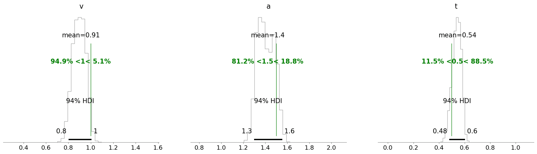
As a last step we can check our posterior distributions. Did all of this actually work out?

NOTE:

The posterior mass here may be somewhat off the mark when comparing to the ground truth parameters. While this hints at a calibration issue, it was conscious approach to trade-off on precision to avoid potentially very long runtimes for this tutorial. We can in general improve the performance of our neural network by training on much more synthetic data (which in real applications is advisable). This would however make running this notebook very cumbersome, which we in turn encourage you to try!

import arviz as az
az.plot_posterior(ddm_blog_traces_numpyro,
                  kind = 'hist',
                  **{'color': 'black', 
                     'histtype': 'step'},
                  ref_val = {'v': [{'ref_val': parameters['v']}],
                             'a': [{'ref_val': parameters['a']}],
                             't': [{'ref_val': parameters['z']}]
                            },
                  ref_val_color = 'green')

array([<Axes: title={'center': 'v'}>, <Axes: title={'center': 'a'}>,
       <Axes: title={'center': 't'}>], dtype=object)

A somewhat long but hopefully rewarding tutorial is hereby finished. We hope you see some potential in this approach. Many extensions are possible, from the choice of neural network architectures to the structure of the PyMC model a plethora of options arise. As a lowest bar, we hope that this may serve you as another take on a tutorial concerning custom distributions in PyMC.

For related tutorials check out:

1. Building blackbox likelihood functions

2. Working with custom distributions

3. Wrapping jax functions into PyTensor Ops

4. ODEs, Bayesian Neural Nets with Flax and PyMC