Bayesian Spatial Modeling for Evaluating Hockey Goaltending Performance
Bayesian Spatial Modeling for Evaluating Hockey Goaltending Performance
December 17, 2025
By Chris Fonnesbeck
Evaluating goalie performance accurately is a challenging task in hockey analytics. Traditional metrics are commonly used due to their simplicity and interpretability: What proportion of shots did the goalie stop (save percentage SV%), and how many goals on average did they allow per game (goals against average GAA)?
However, these metrics have significant limitations, they fail to account for the varying difficulty and types of shots goalies face, and they often conflate goalie skill with other aspects of team defensive performance. As a result, goalies playing behind strong defensive teams may appear better than they truly are, while those facing tougher shot profiles may be unfairly penalized.
To address these limitations, analysts have increasingly turned to more advanced statistical methods. One approach is to apply expected goals (xG) models, which estimate the probability of a shot resulting in a goal based on factors such as shot location, angle, and other predictors. While xG models represent a significant improvement over traditional metrics, they are typically estimated with machine learning methods that provide only point estimates and do not explicitly quantify the uncertainty inherent in estimating player performance.
Bayesian modeling offers an alternative approach that produces probabilistic estimates of goalie skill. This allows us to adjust for shot difficulty and type systematically, providing a more nuanced and accurate evaluation of goalie performance. In this post, we’ll demonstrate how Bayesian modeling can be applied to hockey analytics to estimate goalie skill, adjusting for the type and difficulty of shots faced. We’ll walk through the modeling process step-by-step, clearly explaining each decision and interpreting the results to gain deeper insights into goalie performance.
The Bayesian Advantage in Hockey Analytics
Before diving into the analysis, it’s important to understand why Bayesian methods are uniquely suited for hockey analytics:
1. Uncertainty Quantification: Hockey data are inherently noisy, with small sample sizes and high variability. Bayesian methods provide full posterior distributions rather than point estimates, allowing us to distinguish between genuine skill differences and statistical noise.
2. Hierarchical Modeling: Hockey data has inherent hierarchical structure (players within teams and positions, shots within games, etc.). PyMC excels at modeling these relationships, allowing us to borrow strength across groups while still capturing individual effects.
3. Flexible Model Construction: Rather than forcing our data into restrictive parametric assumptions, PyMC’s probabilistic programming allows us to build models that reflect the actual generative process of hockey events.
4. Principled Model Comparison: Bayesian methods provide robust frameworks for comparing different model formulations, helping us understand which factors truly matter for performance.
5. Computational Efficiency: Modern MCMC algorithms like NUTS, combined with JAX acceleration, make sophisticated spatial modeling computationally feasible even for large hockey datasets.
Throughout this analysis, we’ll see how these advantages translate into practical improvements over traditional hockey metrics.
Data Loading and Preprocessing
To demonstrate the Bayesian modeling approach, we’ll use a dataset containing shot information from the 2023-2024 NHL season.
This dataset comes from MoneyPuck, and includes various features such as shot location, shot type, rebound status, and whether the shot resulted in a goal.
season = 2023
shots = load_shots(DATA_DIR, season)
Dataset loaded successfully:
- Raw dataset: 121,670 shots
- Unique goalies: 99
- Unique shooters: 921
- Total columns: 124
Just to keep things simple, we will filter the data to remove shots on an empty net as well as shots taken during power play or short-handed situations. Further, we will only consider shots from the offensive zone.
After preprocessing:
- Filtered shots: 91,247
- Retention rate: 75.0%
- Removed: Empty net, power play, and non-offensive zone shots
Next, we need to encode the identities of the goalies and shooters.
goalies = (
    ozone_shots.select("goalieNameForShot").unique().to_series().sort().to_list()
)
shooters = ozone_shots.select("shooterName").unique().to_series().sort().to_list()
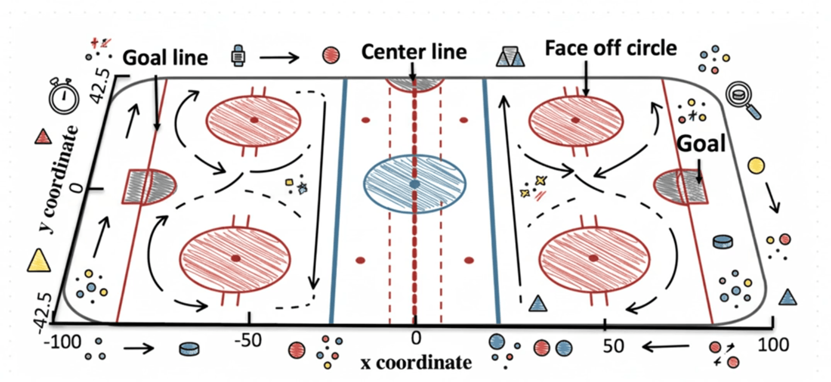
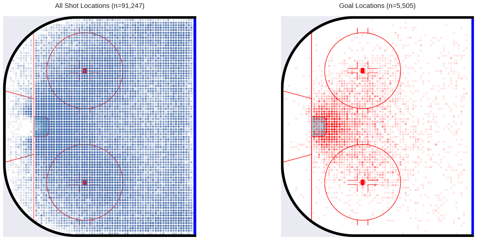
Just to get an idea of what we are dealing with, let’s plot the shot locations in the offensive zone, as well as the locations of shots that resulted in goals.
Understanding Shot Types: The Foundation of Our Analysis
You may have noticed that there are over 90,000 shots in the processed dataset, which will be inconvenient computationally. Let’s break the dataset down by shot type, which we will want to use anyway, since there is a lot of heterogeneity among the shot types.
Understanding shot types is crucial for accurate goalie evaluation. Each type has distinct characteristics that affect both success probability and the skills required to stop them:
1. WRIST: A wrist shot is a quick release shot where the player uses primarily their wrists to propel the puck. It’s a relatively accurate but less powerful shot. Players can maintain better control and disguise the shot’s direction.

2. SLAP: A slap shot is the most powerful shot type where the player raises their stick back and forcefully slaps it against the ice behind the puck, generating maximum force. While powerful, it takes longer to execute and is generally less accurate than other shot types.

3. SNAP: The snap shot combines elements of both wrist and slap shots, offering a quick release with moderate power. The stick briefly leaves the ice surface. It’s faster to execute than a slap shot but delivers more power than a wrist shot.
4. TIP_DEFL: This category combines tip-ins and deflections, where players redirect shots or passes to change the puck’s direction, often surprising the goalie. These shots typically occur very close to the net and rely on timing and hand-eye coordination rather than power.

5. BACK : A backhand shot is taken from the back side of the stick blade, often used when a player’s body position prevents a forehand shot. While generally less powerful than forehand shots, backhands can be difficult for goalies to read.
6. WRAP: A wrap-around shot occurs when a player skates behind the net and attempts to score by quickly wrapping the puck around the post before the goalie can move into position. These shots rely on speed and catching the goalie out of position.
Each shot type tends to be used in different game situations and from different locations on the ice.

While this shows the distribution of shots by type, the distribution of goals over space is quite different, at least for some shot types.
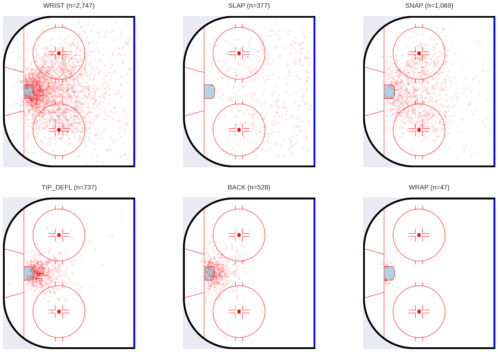
From the above, we can see that different shot types are taken from different locations on the ice, with different degrees of success. We will use this information to inform our model.
Let’s then encode the shot types as a categorical variable.
shot_types = ozone_shots.select("shotType").unique().to_series().sort().to_list()

# Cast to Enum and then encode to integers
encoded_shots = ozone_shots.with_columns(
    [
        pl.col("shotType")
        .cast(pl.Enum(shot_types))
        .to_physical()
        .alias("shotType_idx")
    ]
).select(["shotType_idx", "shotType"])
Building Our Bayesian Models: An Iterative Approach
It’s clear from these plots that shot location has a strong effect on the probability of a goal. So a reasonable starting point is to model the goal rate simply as a function of where the shot occurs. Looking at the available data, one approach would be to use shotDistancemand shotAngle as predictors, where we expect shots that are both closer to the goal and from the middle of the ice to be more likely to result in a goal.
The Spatial Approach: Gaussian Process Priors
I’m going to take a more explicitly spatial approach, and use shot location to inform a Gaussian process prior on the goal rate. A Gaussian Process (GP) is a powerful non-parametric model that defines a probability distribution over functions. It’s particularly well-suited for spatial data because it inherently models the spatial correlation: points closer together are assumed to have more similar values. This relationship is captured by a kernel function, which defines the covariance between any two points based on their distance. Using a GP allows us to not only model the observed goal rates at observed shot locations but also to predict the goal rate and its uncertainty across the entire ice surface. This prediction process, leveraging the spatial correlation structure learned by the GP to interpolate values at unobserved locations, is known as Kriging.
Model 1: Baseline Spatial Model
As a baseline, we will fit a model that is just a function of shot location. Moreover, we will restrict the dataset to one shot type (wrist shots) during the 2023-2024 season.
fitting_subset = ozone_shots.filter(pl.col("shotType") == "WRIST")
fitting_subset.shape
[51022, 134]
The model implements a two-dimensional Gaussian Process (GP) prior on the log-odds of scoring. The GP is defined by two components:
- A mean function m(x) that specifies the expected value at any location x
- A covariance function (or kernel) k(x, x′) that defines how correlated function values are at different locations
The covariance function is the core component of a Gaussian Process—it encodes our assumptions about how shot danger varies spatially. More specifically, it quantifies the similarity between goal probabilities at any two points based on their distance.
For this analysis, we use the Matern52 (also written as Matérn-5/2), a member of the Matérn family characterized by a smoothness parameter ν = 5/2. The Matern52 covariance function is defined as:
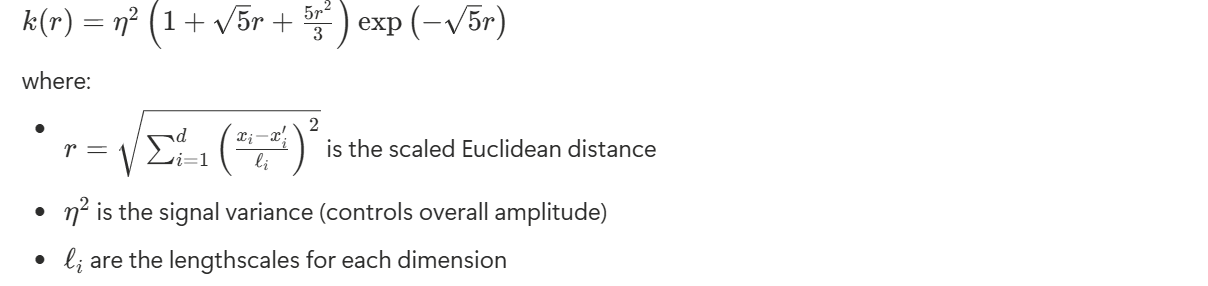
The Matérn-5/2 is one of many possible choices of covariance function. It is appropriate here because it balances several desirable properties:
- Smoothness: Twice differentiable, producing realistic spatial patterns—shot danger changes smoothly across the ice, not in abrupt jumps
- Interpretability: The lengthscale ℓ has a clear interpretation—it’s roughly the distance at which correlation drops to about 1/3 (or e⁻¹)
- Flexibility: Can capture local variation while allowing for global trends
- Computational stability: More numerically stable than the exponential quadratic (a typical default) kernel for many spatial problems
Just to make this concrete, here are a few draws from Gaussian processes using the Matérn-5/2, with a range of length scale parameters:
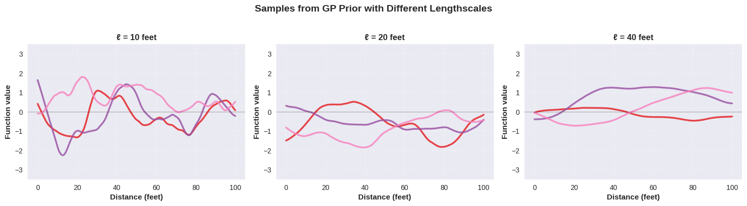
The GP generates a latent value that represents the log-odds of scoring given shot location coordinates x and y. The probability of a goal is modeled through a logit link function. The likelihood function assumes each shot outcome follows a Bernoulli distribution with success probability probability pi =σ(f(xi,yi)), where σ is the sigmoid function. The Gaussian Process prior uses a Matern52 kernel with lengthscale parameters ℓx and ℓy to capture spatial correlation, an amplitude parameter η to control overall variation, and a constant mean function μ = −3 on the log-odds scale (since we would expect regions with no shot data to be areas of low scoring probability).

Since we have a lot of data, even in the shot-type subset we are working with, using exact Gaussian processes will be computationally expensive. Instead, we will use the Hilbert Space Gaussian Process (HSGP) approximation, which allows us to scale GP inference to larger datasets by projecting the GP onto a finite set of basis functions. This approach significantly reduces the computational burden while still capturing the essential spatial structure of the data.
The key decision when using HSGP is the number of basis functions to use in each dimension (m) and the boundary of the compact domain on which the kernel approximation is based ( c ). These hyperparameters control the fidelity of the approximation—the higher the values, the closer the approximation is to the true GP, but at increased computational cost. We can use the approx_hsgp_hyperparams utility from PyMC to help select appropriate values based on the range of our data and expected lengthscales.
m_approx, c_approx = pm.gp.hsgp_approx.approx_hsgp_hyperparams(
    x_range=[
        fitting_subset.select("x_centered").min().item(),
        fitting_subset.select("x_centered").max().item(),
    ],
    lengthscale_range=[10, 50],
    cov_func="Matern52",
)

(m_approx, c_approx)
The larger m and c are, the more computationally expensive the model becomes, so we need to balance accuracy with efficiency. The value for c essentially determines the effective range of the basis functions, and is interpreted as multiples of the range of the fitting dataset.
Let’s see how this all fits into the model.
Aside from selecting the HSGP hyperparameters, an important consideration is the specification of prior distributions for the covariance function parameters. We will use weakly informative priors to allow the data to inform the length scale and amplitude of the Gaussian Process while preventing extreme values that could destabilize inference. For example, we placed an Exponential prior on the amplitude parameter (eta_xy) to encourage moderate variability in the latent function, and a maximum entropy Inverse Gamma prior on the length scale parameters (ell_xy) to favor reasonable spatial correlation ranges without being overly restrictive.
Just as approx_hsgp_hyperparams helped us specify HSGP hyperparameters, we can use another utility to parameterize our GP priors. The maxent function provided by the PreliZ library (aliased by pz) allows us to define maximum entropy priors given quantile constraints, which is useful for setting priors that reflect our domain knowledge without being overly prescriptive.
ell_xy = pz.maxent(
    pz.InverseGamma(), 10, 50, 0.95, plot=False
).to_pymc("ell_xy", shape=2)
This will create an inverse-gamma prior with 95% of the probability between length scales of 10 and 50 feet. Notice that shape=2, since we will have separate length scale parameters for the x and y dimensions.
The rest of the model specification directly reflects our mathematical formulation above.
coords = {"shot": np.arange(fitting_subset.shape[0])}

def baseline_xg_model(data, coords, m, c):
    with pm.Model(coords=coords) as model:
        # Data nodes
        goal = pm.Data("goal", data.select("goal").to_numpy().squeeze())
        shot_xy = pm.Data(
            "shot_xy",
            data.select(["x_centered", "y"]).to_numpy().astype(np.float32),
        )

        # GP hyperparameters
        eta_xy = pm.Exponential("eta_xy", scale=1)
        ell_xy = pz.maxent(pz.InverseGamma(), 10, 50, 0.95, plot=False).to_pymc(
            "ell_xy", shape=2
        )

        # Covariance function
        cov_func_xy = eta_xy**2 * pm.gp.cov.Matern52(input_dim=2, ls=ell_xy)

        # Latent HSGP
        gp_xy = pm.gp.HSGP(
            m=[m, m],
            c=c,
            mean_func=pm.gp.mean.Constant(-3),
            cov_func=cov_func_xy,
        )
        f_xy = gp_xy.prior("f_xy", X=shot_xy)

        # Likelihood function
        pm.Bernoulli("obs_goals", logit_p=f_xy, observed=goal, dims="shot")

    return model

baseline_xg = baseline_xg_model(fitting_subset, coords, m=m_approx, c=c_approx)

baseline_xg
We fit the model using Markov Chain Monte Carlo (MCMC) sampling. Specifically, we use the NUTS sampler implemented in nutpie, which can be accelerated using the JAX backend (particularly if we have a GPU).
baseline_xg_trace = sample_model(
    baseline_xg,
    filename="baseline",
    use_cached=USE_CACHED,
    backend=BACKEND,
    season=season,
)
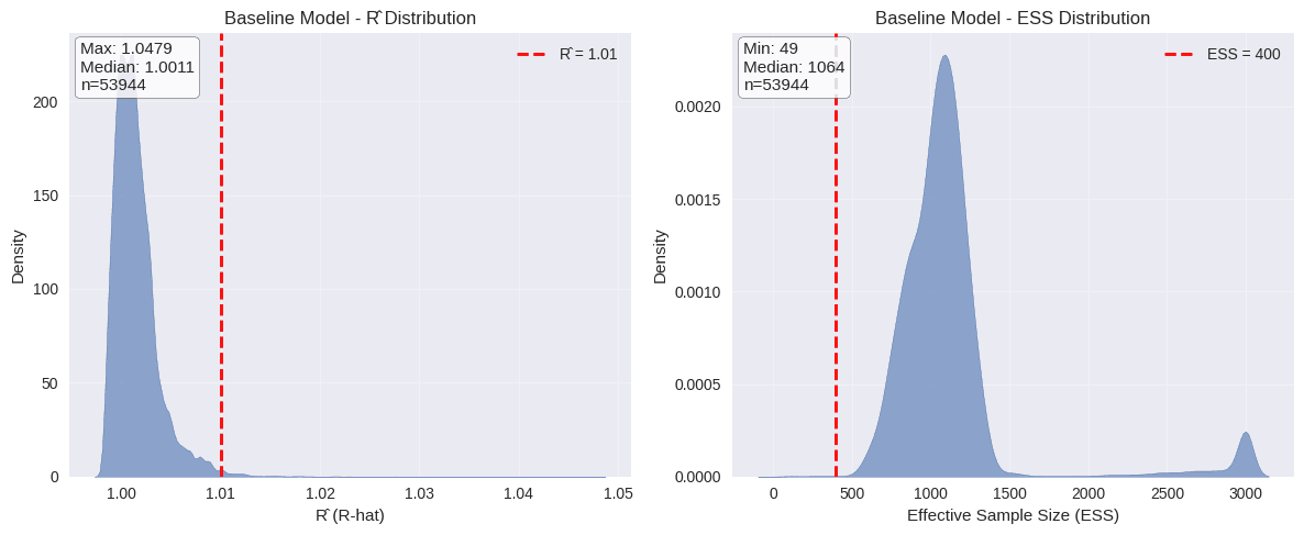
Let’s do a quick model check: first, plotting distributions of R-hat and effective sample size for all parameters shows the model has converged well, with R-hat values close to 1 and adequate effective sample sizes across most parameters.
plot_mcmc_diagnostics(baseline_xg_trace, "Baseline Model")
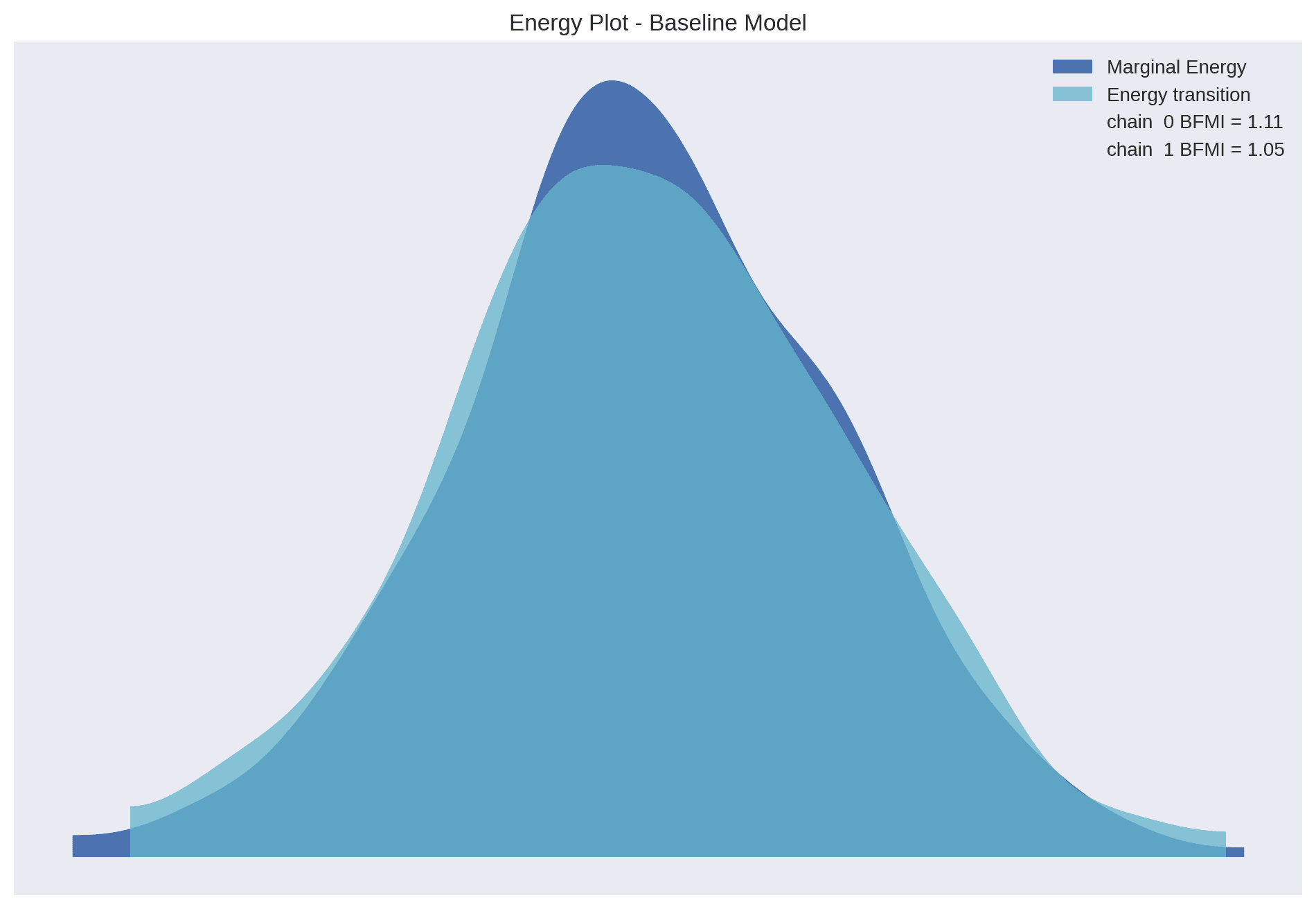
 Further, the strong overlap between transitional energy and marginal energy by the NUTS sampling algorithm implies that the sampler was able to efficiently explore the posterior distribution without getting stuck in local modes. This is a good sign that our model is well-specified and that the sampling process was effective.
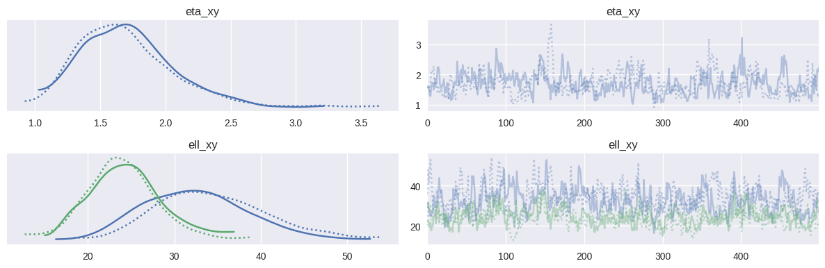
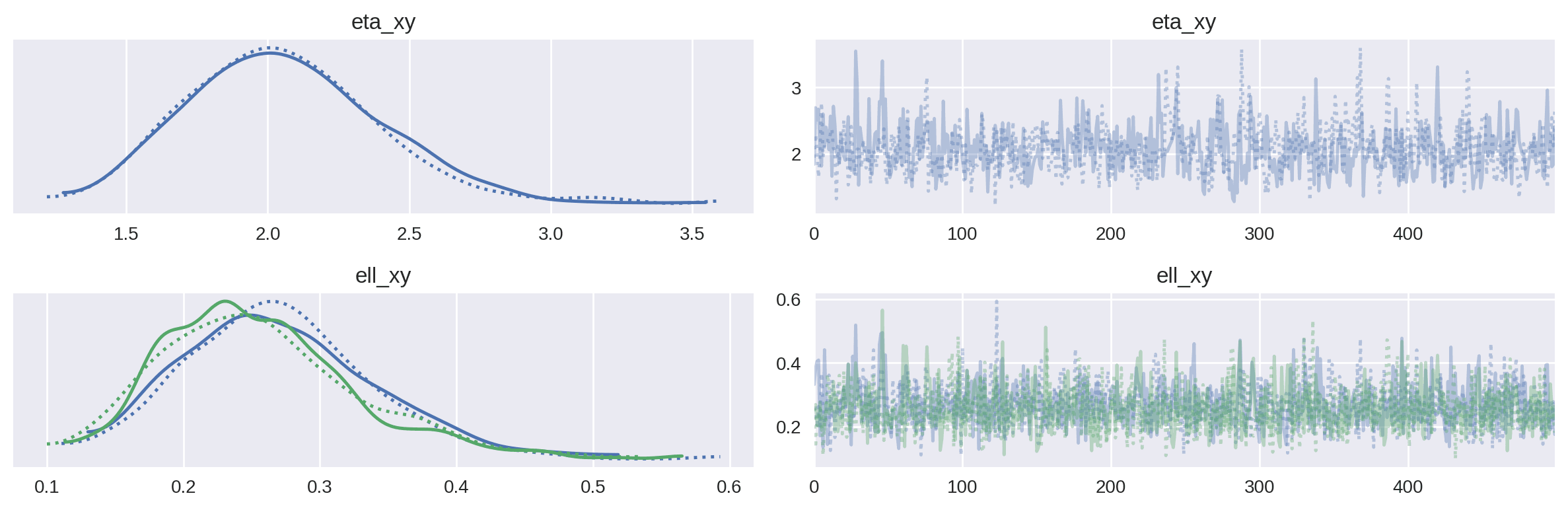
Looking at the posterior distributions of the covariance function parameters, we can see that the length scales are in the 30-40 range for the x-axis (length of the rink) and the 20-30 range for the y-axis (rink width), indicating the distances over which we expect shot quality to vary spatially. The signal variance parameter (η) indicates the overall variability in shot quality across the ice.
_ = az.plot_trace(baseline_xg_trace, var_names=["eta_xy", "ell_xy"])
plt.tight_layout()
plt.gcf()
Now that the GP model is fit, we can use the model to predict across the entire offensive zone. Rather than using the observed shot locations, we set the input data to be a grid of points–one of the advantages of Gaussian distributions (and hence, Gaussian processes) is that it is easy to generate conditional distributions for abitrary points. We can sample from the posterior predictive distribution across this grid to obtain a surface of expected goals.
with baseline_xg:
    pm.set_data(
        {
            "shot_xy": grid_data.astype(np.float32),
        }
    )
    baseline_xg_pred = sample_posterior_predictive(
        baseline_xg_trace,
        filename="baseline_pred",
        var_names=["f_xy"],
        predictions=True,
    )
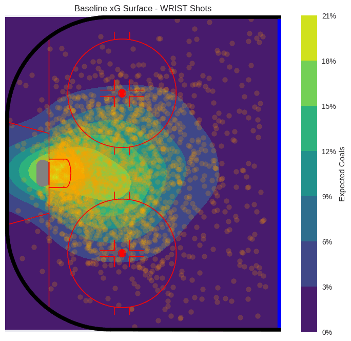
The xG surface shows the typical “danger zone” in hockey – the slot area in front of the net, with probabilities quickly dropping beyond the faceoff dots. Notice there is a slight asymmetry favoring the right side of the ice (from the goalie’s perspective), which may reflect the fact that 90% of goalies’ glove side is on the left.
plot_rink_heatmap(
    grid_x,
    grid_y,
    sigmoid(
        baseline_xg_pred.predictions["f_xy"].mean(dim=["draw", "chain"]).values
    ),
    title=f"Baseline xG Surface - {shot_type} Shots",
    cmap="viridis",
    fitting_data=fitting_subset,
)
Model 2: Coordinate Warping
As this is a baseline model, it is pretty easy to spot flaws and areas for improvement. For instance, based on the probability contours, the probability of scoring from directly behind the net is the same as from the slot near the top of the circle! Since these are wrist shots and not wrap-arounds or “Michigans” this is not credible.
This is due to the fact that goal scoring opportunities are not isotropic across the ice surface. Shots taken from near the goal line or behind the net are not nearly as dangerous as those taken from in front of the net. More generally, the quality of goal scoring opportunities change more rapidly with location in the space around the goal and goal line than in areas farther away.
One approach for handling this heterogeneity is to use coordinate warping, where we transform the input coordinates based on their distance from the goal. This effectively allows the Gaussian Process to have a spatially-varying lengthscale, capturing the idea that shot quality changes more rapidly in certain areas of the ice.
We will use an arcsinh (inverse hyperbolic sine) warping function on the input coordinates to create a spatially-varying effective lengthscale. The arcsinh transformation has desirable properties: it behaves approximately linearly near the origin (close to the goal) and logarithmically at larger distances. This means shot quality can vary rapidly near the goal where small position changes matter greatly, while the model smooths over larger distances away from the net where positional differences are less critical. The transformation is applied radially as:

where r is the distance from the goal, δ is an offset parameter (set to 5 feet) that ensures a minimum effective lengthscale near the crease, and α is a scale parameter (set to 20 feet) that controls the transition between linear and logarithmic behavior.
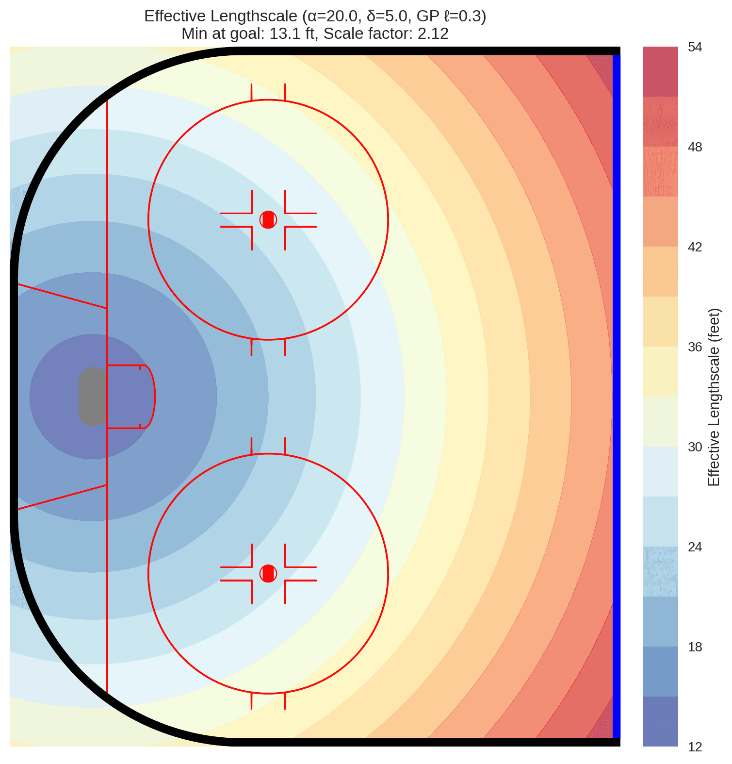
We use fixed hyperparameters for the warping function (α=20, δ=5) rather than estimating them, as this provides a stable coordinate transformation that allows the Gaussian Process to learn the spatial correlations effectively on the warped domain. This approach avoids the computational complexity and potential identifiability issues of learning the warping parameters simultaneously with the GP.
def compute_warp_scale(data, warp_alpha=20.0, delta=5.0):
    """Compute normalization scale for warped coordinates.

    Returns a scale factor that normalizes warped coordinates to ~[-1, 1]
    range. The delta parameter adds an offset to ensure minimum effective
    lengthscale near the goal (smooths out the crease area).
    """
    x_max = np.abs(data.select("x_centered").to_numpy()).max()
    y_max = np.abs(data.select("y").to_numpy()).max()
    r_max = np.sqrt(x_max**2 + y_max**2)
    return float(np.arcsinh((r_max + delta) / warp_alpha))

def warped_input_xg_model(data, coords, m=None, c=None):
    """Build xG model with warped input coordinates using Arcsinh warping."""
    warp_alpha = 20.0
    delta = 5.0  # Radius offset to ensure a minimum effective lengthscale
    scale_factor = compute_warp_scale(data, warp_alpha=warp_alpha, delta=delta)

    # Calculate HSGP params for normalized domain if not provided
    if m is None or c is None:
        m_est, c_est = pm.gp.hsgp_approx.approx_hsgp_hyperparams(
            x_range=[-1.1, 1.1], lengthscale_range=[0.1, 0.6], cov_func="Matern52"
        )
        m = int(np.sqrt(m_est)) if m is None else m
        c = c_est if c is None else c

    with pm.Model(coords=coords) as model:
        goal = pm.Data("goal", data.select("goal").to_numpy().squeeze())
        shot_xy = pm.Data(
            "shot_xy",
            data.select(["x_centered", "y"]).to_numpy().astype(np.float32),
        )

        # Warp coordinates: arcsinh((r + delta)/alpha)
        # Delta offset ensures minimum effective lengthscale near the goal
        r = pm.math.sqrt(shot_xy[:, 0] ** 2 + shot_xy[:, 1] ** 2 + 1e-6)
        r_effective = r + delta

        # Note: No beta_warp. We let the GP learn the amplitude via eta_xy/ell_xy
        # We just provide the non-linear shape transformation.
        r_warped = pm.math.arcsinh(r_effective / warp_alpha)

        # Direction vector (unchanged)
        # x_warped = x * (r_warped / r)
        shot_xy_warped = pm.math.stack(
            [shot_xy[:, 0] * r_warped / r, shot_xy[:, 1] * r_warped / r], axis=1
        )

        # Normalize to fixed domain for HSGP
        shot_xy_normalized = shot_xy_warped / scale_factor

        # GP with priors scaled to normalized space
        eta_xy = pm.Exponential("eta_xy", scale=1)
        ell_xy = pz.maxent(pz.InverseGamma(), 0.1, 0.5, 0.95, plot=False).to_pymc(
            "ell_xy", shape=2
        )

        cov_func_xy = eta_xy**2 * pm.gp.cov.Matern52(input_dim=2, ls=ell_xy)
        gp_xy = pm.gp.HSGP(
            m=[m, m], c=c, mean_func=pm.gp.mean.Constant(-3), cov_func=cov_func_xy
        )
        f_xy = gp_xy.prior("f_xy", X=shot_xy_normalized)

        pm.Bernoulli("obs_goals", logit_p=f_xy, observed=goal, dims="shot")

    return model

# Let function calculate parameters dynamically
warped_input_xg = warped_input_xg_model(fitting_subset, coords)
warped_input_xg_trace = sample_model(
    warped_input_xg,
    filename="warped_input",
    use_cached=USE_CACHED,
    backend=BACKEND,
    season=season,
)

with warped_input_xg:
    pm.set_data({"shot_xy": grid_data.astype(np.float32)})
    warped_pred = sample_posterior_predictive(
        warped_input_xg_trace,
        filename="warped_input_pred",
        var_names=["f_xy"],
        predictions=True,
    )
Note that the estimated length scale parameters are now on the warped domain.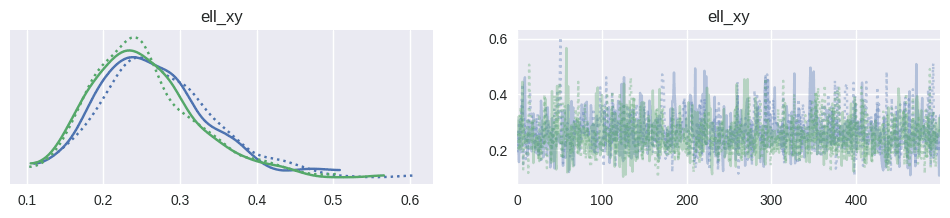
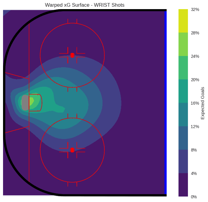
The resulting xG surface is now a little more dynamic in the areas around the goal.
plot_rink_heatmap(
    grid_x,
    grid_y,
    sigmoid(warped_pred.predictions["f_xy"].mean(dim=["draw", "chain"]).values),
    title=f"Warped xG Surface - {shot_type} Shots",
    cmap="viridis",
    fitting_data=fitting_subset,
    show_goals=False,
)
Model 3: Incorporating Contextual Effects
Beyond shot location, its easy to imagine other factors that influence the probability of a goal. There is a lot of additional context that determines whether or not any given shot is dangerous from a particular location. Let’s expand the model by incorporating additional predictors.
Even in our limited dataset, there are a few candidate variables that should affect the quality of a shot:
- Off-wing shots: Shots from a player’s non-preferred side
- Rebounds: Shots that occur shortly after another shot or save
- Rebound angle: High-angle rebounds force the goalie to move laterally quickly

To keep things simple, let’s add a rebound effect; just a simple indicator for shots that are rebounds off of the goaltender or goalpost from a previous shot.
Ordinarily, we might treat this variable as simple fixed effect, influencing the prediction in a constant, additive fashion. However, its easy to imagine that a rebound creates a better goal-scoring opportunity in some locations of the ice (e.g. in the slot) relative to others.
The fact that we are using latent Gaussian processes means that we can combine them additively (or multiplicatively, if we wish), so we’ll include a rebound effect as a separate Gaussian Processes. This allows us to capture how a rebound may be more or less important in different areas of the ice.
def covariate_xg_model(data, coords, m=None, c=None):
    warp_alpha = 20.0
    delta = 5.0
    scale_factor = compute_warp_scale(data, warp_alpha=warp_alpha, delta=delta)

    if m is None or c is None:
        m_est, c_est = pm.gp.hsgp_approx.approx_hsgp_hyperparams(
            x_range=[-1.1, 1.1], lengthscale_range=[0.1, 0.6], cov_func="Matern52"
        )
        m = int(np.sqrt(m_est)) if m is None else m
        c = c_est if c is None else c

    with pm.Model(coords=coords) as model:
        # Add rebound indicator
        rebound = pm.Data(
            "rebound",
            data.select("shotAnglePlusRebound").to_numpy().squeeze() > 0,
        )
        goal = pm.Data("goal", data.select("goal").to_numpy().squeeze())
        shot_xy = pm.Data(
            "shot_xy",
            data.select(["x_centered", "y"]).to_numpy().astype(np.float32),
        )

        r = pm.math.sqrt(shot_xy[:, 0] ** 2 + shot_xy[:, 1] ** 2 + 1e-6)
        r_effective = r + delta
        r_warped = pm.math.arcsinh(r_effective / warp_alpha)

        shot_xy_warped = pm.math.stack(
            [shot_xy[:, 0] * r_warped / r, shot_xy[:, 1] * r_warped / r], axis=1
        )

        shot_xy_normalized = shot_xy_warped / scale_factor

        eta_xy = pm.Exponential("eta_xy", scale=1)
        ell_xy = pz.maxent(pz.InverseGamma(), 0.1, 0.5, 0.95, plot=False).to_pymc(
            "ell_xy", shape=2
        )

        cov_func_xy = eta_xy**2 * pm.gp.cov.Matern52(input_dim=2, ls=ell_xy)
        gp_xy = pm.gp.HSGP(
            m=[m, m], c=c, mean_func=pm.gp.mean.Constant(-3), cov_func=cov_func_xy
        )
        f_xy = gp_xy.prior("f_xy", X=shot_xy_normalized)

        # Rebound GP
        eta_rebound = pm.Exponential("eta_rebound", scale=1)
        ell_rebound = pz.maxent(
            pz.InverseGamma(), 0.1, 0.5, 0.95, plot=False
        ).to_pymc("ell_rebound", shape=2)
        cov_func_rebound = eta_rebound**2 * pm.gp.cov.Matern52(
            input_dim=2, ls=ell_rebound
        )
        gp_rebound = pm.gp.HSGP(m=[m, m], c=c, cov_func=cov_func_rebound)
        f_rebound = gp_rebound.prior("f_rebound", X=shot_xy_normalized)

        logit_p = pm.Deterministic("logit_p", f_xy * (1 + rebound * f_rebound))

        pm.Bernoulli("obs_goals", logit_p=logit_p, observed=goal, dims="shot")

    return model

covariate_xg = covariate_xg_model(fitting_subset, coords)

covariate_xg
An important modeling choice is the multiplicative interaction between the shot location effect and the rebound effect in the model specification: logit_p = f_xy * (1 + rebound * f_rebound). This multiplicative structure allows the rebound effect to scale proportionally with the baseline shot quality rather than adding a constant boost everywhere. Conceptually, this makes sense: a rebound in the slot (where f_xy is already high) should have a larger absolute impact than a rebound from a low-danger area like the corner. The multiplicative kernel effectively makes the rebound GP modulate the strength of the spatial pattern, capturing how rebounds amplify existing scoring opportunities rather than creating uniform increases across the ice. This is in contrast to a simple additive model (f_xy + rebound * f_rebound) which would assume rebounds add the same absolute benefit regardless of location.
covariate_xg_trace = sample_model(
    covariate_xg,
    filename="covariate",
    use_cached=USE_CACHED,
    backend=BACKEND,
    season=season,
)
az.plot_trace(covariate_xg_trace, var_names=["eta_xy", "ell_xy"])
plt.tight_layout()
plt.show()
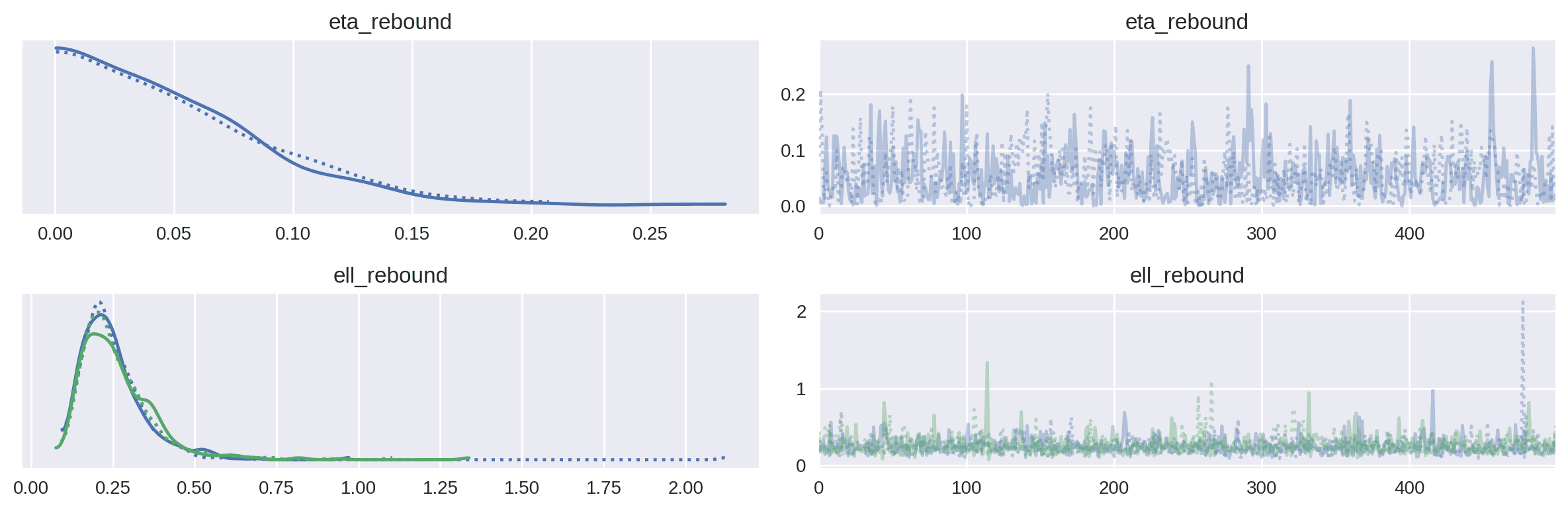
az.plot_trace(covariate_xg_trace, var_names=["eta_rebound", "ell_rebound"])
plt.tight_layout()
plt.show()
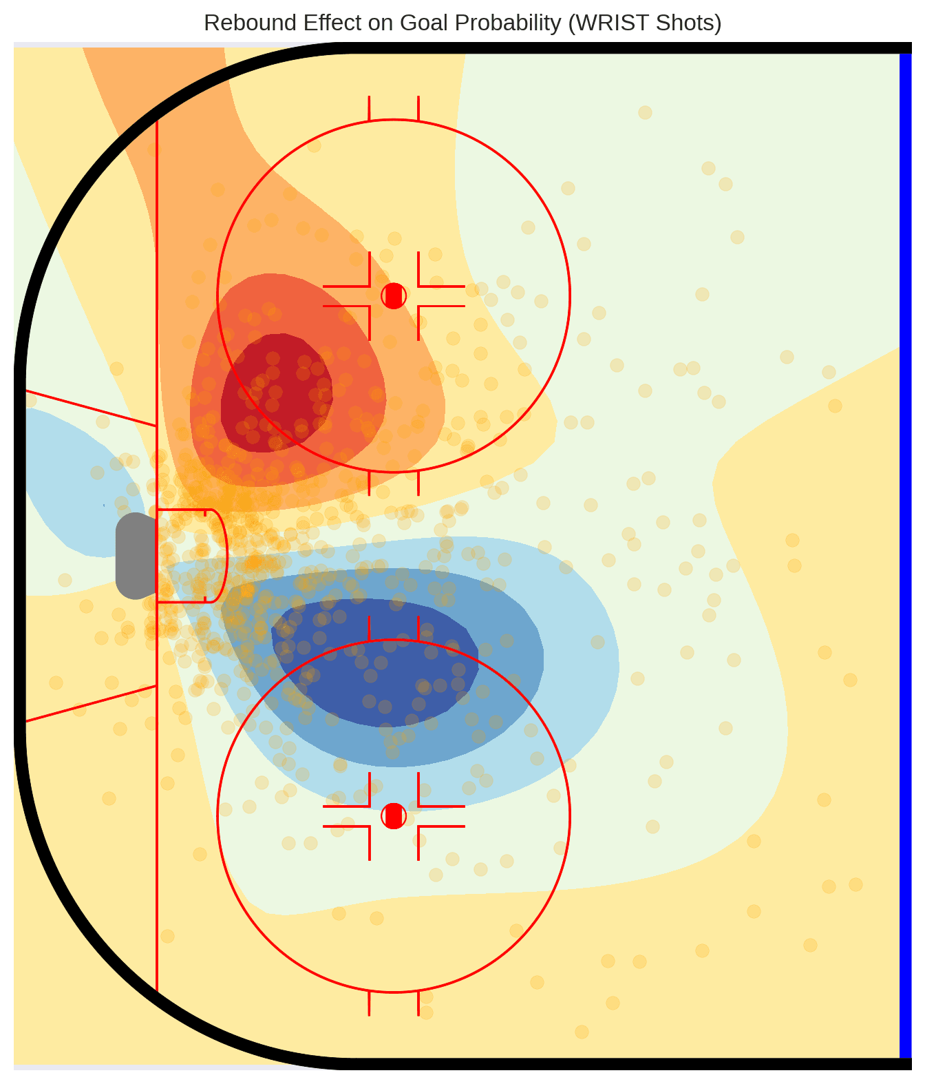
Visualizing Contextual Effects
We can generate predictions from this covariate model to see how rebound effects vary spatially. Red areas are positive relative to non-rebound shots and blue negative.
Model 4: Hierarchical shooter effects
While we could find additional covariates to account for variation in goal probability, let’s move on to address heterogeneity of shot quality due to shooter talent. Our current model assumes that, given location and shot type, the goal probability is uniform. Yet we know that some players’ shots are better than others–Steve Stamkos’ wrist shot is more dangerous than Tyler Myers’, for example. Since we are ultimately looking to evaluate goaltender effectiveness, its worth adjusting for the relative quality of the shooters taking the shots.
Ideally we would have data on puck velocity and other shot characteristics to further refine our estimates of shot quality. However, such data is not consistently available in the public domain across all leagues and seasons. Instead, we can use a hierarchical modeling approach to estimate shooter-specific random effects that capture unobserved shooter skill differences.
def hierarchical_xg_model(data, coords, m=None, c=None):
    warp_alpha = 20.0
    delta = 5.0
    scale_factor = compute_warp_scale(data, warp_alpha=warp_alpha, delta=delta)

    if m is None or c is None:
        m_est, c_est = pm.gp.hsgp_approx.approx_hsgp_hyperparams(
            x_range=[-1.1, 1.1], lengthscale_range=[0.1, 0.6], cov_func="Matern52"
        )
        m = int(np.sqrt(m_est)) if m is None else m
        c = c_est if c is None else c

    with pm.Model(coords=coords) as model:
        rebound = pm.Data(
            "rebound",
            data.select("shotAnglePlusRebound").to_numpy().squeeze() > 0,
        )
        goal = pm.Data("goal", data.select("goal").to_numpy().squeeze())
        shot_xy = pm.Data(
            "shot_xy",
            data.select(["x_centered", "y"]).to_numpy().astype(np.float32),
        )
        # Shooter index values
        shooter_idx = pm.Data(
            "shooter_idx", data.select("shooter_idx").to_numpy().squeeze()
        )

        r = pm.math.sqrt(shot_xy[:, 0] ** 2 + shot_xy[:, 1] ** 2 + 1e-6)
        r_effective = r + delta
        r_warped = pm.math.arcsinh(r_effective / warp_alpha)
        shot_xy_warped = pm.math.stack(
            [shot_xy[:, 0] * r_warped / r, shot_xy[:, 1] * r_warped / r], axis=1
        )

        shot_xy_normalized = shot_xy_warped / scale_factor

        eta_xy = pm.Exponential("eta_xy", scale=1)
        ell_xy = pz.maxent(pz.InverseGamma(), 0.1, 0.5, 0.95, plot=False).to_pymc(
            "ell_xy", shape=2
        )
        cov_func_xy = eta_xy**2 * pm.gp.cov.Matern52(input_dim=2, ls=ell_xy)
        gp_xy = pm.gp.HSGP(
            m=[m, m], c=c, mean_func=pm.gp.mean.Constant(-3), cov_func=cov_func_xy
        )
        f_xy = gp_xy.prior("f_xy", X=shot_xy_normalized)

        eta_rebound = pm.Exponential("eta_rebound", scale=1)
        ell_rebound = pz.maxent(
            pz.InverseGamma(), 0.1, 0.5, 0.95, plot=False
        ).to_pymc("ell_rebound", shape=2)
        cov_func_rebound = eta_rebound**2 * pm.gp.cov.Matern52(
            input_dim=2, ls=ell_rebound
        )
        gp_rebound = pm.gp.HSGP(m=[m, m], c=c, cov_func=cov_func_rebound)
        f_rebound = gp_rebound.prior("f_rebound", X=shot_xy_normalized)

        # Non-centered shooter random effect
        s_epsilon = pm.HalfNormal("s_epsilon", sigma=0.5)
        z_epsilon = pm.Normal("z_epsilon", dims="shooter")

        logit_p = pm.Deterministic(
            "logit_p",
            f_xy * (1 + rebound * f_rebound) + s_epsilon * z_epsilon[shooter_idx],
        )

        pm.Bernoulli("obs_goals", logit_p=logit_p, observed=goal, dims="shot")

    return model

hierarchical_xg = hierarchical_xg_model(hierarchical_subset, coords)
hierarchical_xg_trace = sample_model(
    hierarchical_xg,
    filename="hierarchical",
    use_cached=USE_CACHED,
    backend=BACKEND,
    season=season,
)
Shooter Quality Effects
Having fit the model, let’s peek at the top- and bottom-5 shooters with the highest and lowest estimated effects, respectively, on goal probability:
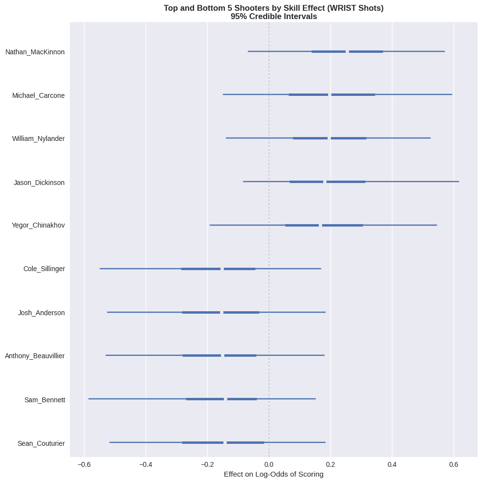
These shooter effects represent the average impact on log-odds of scoring, controlling for shot location, rebounding status, and other contextual factors. Positive values indicate shooters whose shots are more dangerous than average from the same locations. Nathan MacKinnon is at the top of the list, which is a promising sign!
There are a variety of other factors that could be incorporated as a hierarchical random effect. For example, rink effects comprise a suite of unmeasured variables that could influence shooting performance, such as the quality of the ice surface, the presence of fans, and the average temperature and humidity of the arena.
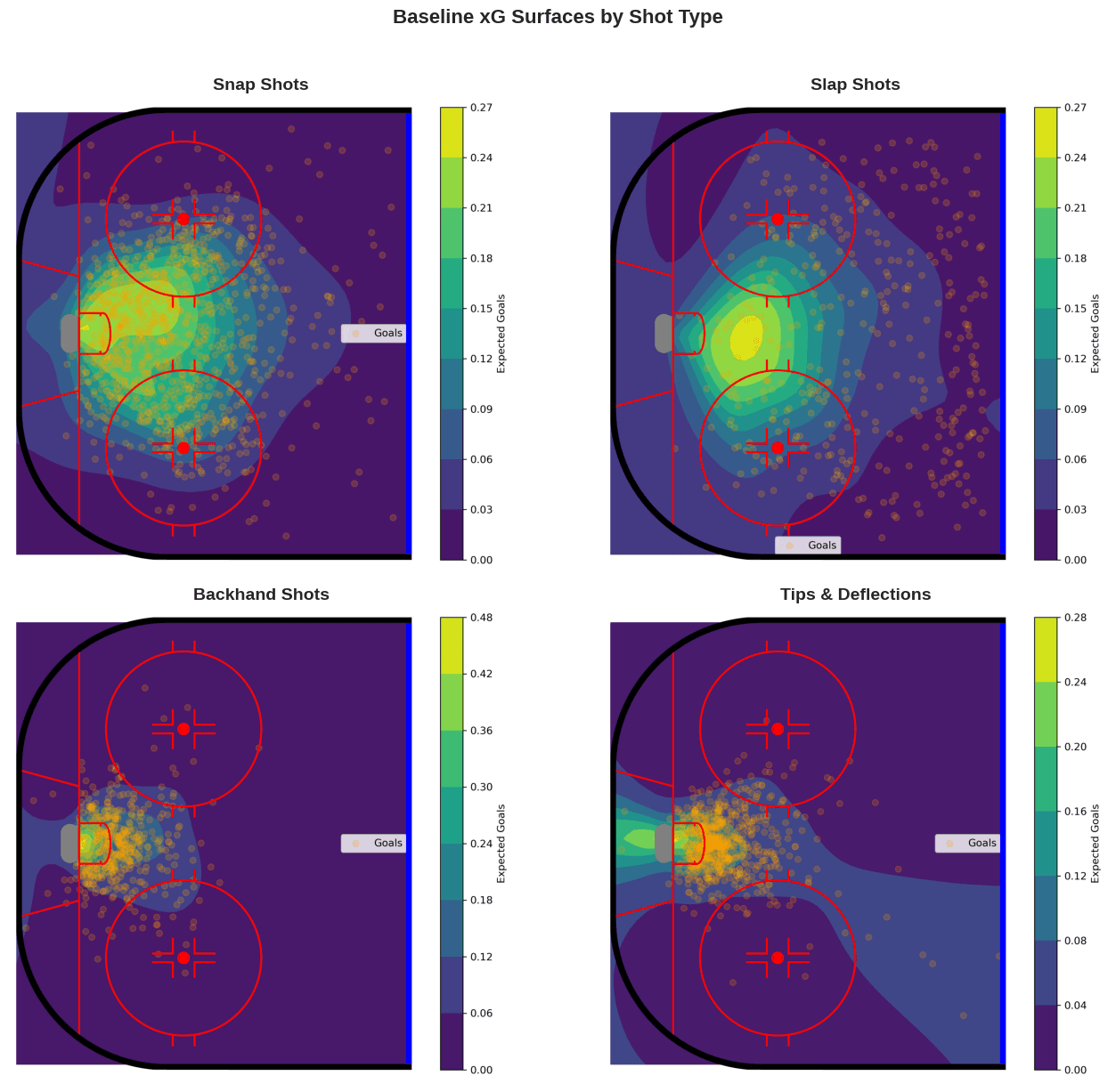
Baseline xG Surfaces for Other Shot Types
While we’ve focused on wrist shots to illustrate the modeling approach, the same methodology applies to most of the shot types–the exception being wraparound shots, which do not have a meaningful spatial distribution. The distribution of goal probability across the offensive zone varies considerably across shot types, reflecting differences in shot mechanics, typical shooting distances, and often goaltender positioning. Below are the baseline xG surfaces for four additional shot types: snap shots, slap shots, backhands, and tips/deflections.
Its worth noting that despite using approximate HSGP models in place of exact Gaussian processes, running the model over all shot types is computationally demanding. Taking advantage of GPU acceleration via JAX reduced runtime from more than a day to just over an hour.
In the absence of accelerated hardware, another solution is to look to faster, approximate methods of model fitting, and not slavishly commit to Markov Chain Monte Carlo (MCMC) as I did here. For example, variational inference can often provide a reasonable approximation to the posterior in a fraction of the time. PyMC supports multiple variational inference algorithms, each of which can be applied using the pm.fit() function.
# Using ADVI
with model:
    approx = pm.fit(method="advi", n=30_000)
    trace = approx.sample(1000)
The tradeoff is that variational methods fit approximate distributions to the true posterior rather than trying to work with the true posterior, which often underestimates uncertainty in complex or multimodal distributions.
Estimating GSAx
Once we are satisfied with our model for one shot type, we can apply it to each of the remaining categories. If the model is general enough, the same model could plausibly be re-used, or we may carefully customize the model to each type according to its characteristics. For example, wrap-around shots are so spatially restricted to a few feet of ice on either side of the goal that a spatial model may be unnecessary. At the very least, we need to re-estimate the model parameters for each shot type to capture their unique spatial and contextual patterns; for example, rebounds will matter more for some shot types than other.
Once we are able to estimate goal probability for all shot types, we can use our set of models to evaluate goal performance, using a metric like Goals Saved Above Expected (GSAx).
Calculating GSAx
GSAx quantifies how many goals a goalie prevented (or allowed) relative to expectation based on shot quality. For a goalie facing shots indexed by i = 1, …, n, where xGi is the expected goal probability for shot i and yi is the actual outcome, GSAx is computed as:

The first term is the total expected goals the goalie should have allowed based on shot quality, and the second term is the actual goals allowed. A positive GSAx indicates the goalie saved more goals than expected (better than average performance), while a negative GSAx indicates they allowed more goals than expected (worse than average).
In our Bayesian framework, we have posterior samples of the expected goal probability xGi(s) for each shot i and each posterior sample s = 1, …, S. This yields a posterior distribution of GSAx:

From these posterior samples, we compute the posterior mean as our point estimate and credible intervals to quantify uncertainty. This approach naturally propagates uncertainty from the xG model through to the goalie evaluation, acknowledging that we don’t know the true expected goal probabilities with certainty.
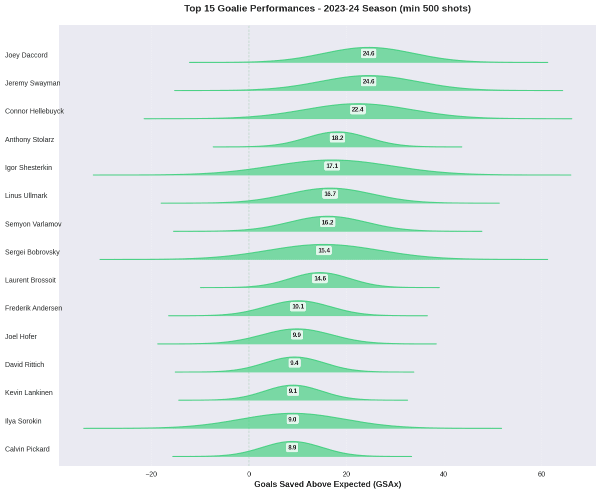
Top Performers: Elite Goaltending in 2023-24
Let’s examine the top-performing goalies, focusing on those with substantial playing time to ensure meaningful comparisons:
Poor Performers: Worst Goalie Performances in 2023-24
Now let’s examine the worst goalies by GSAx:
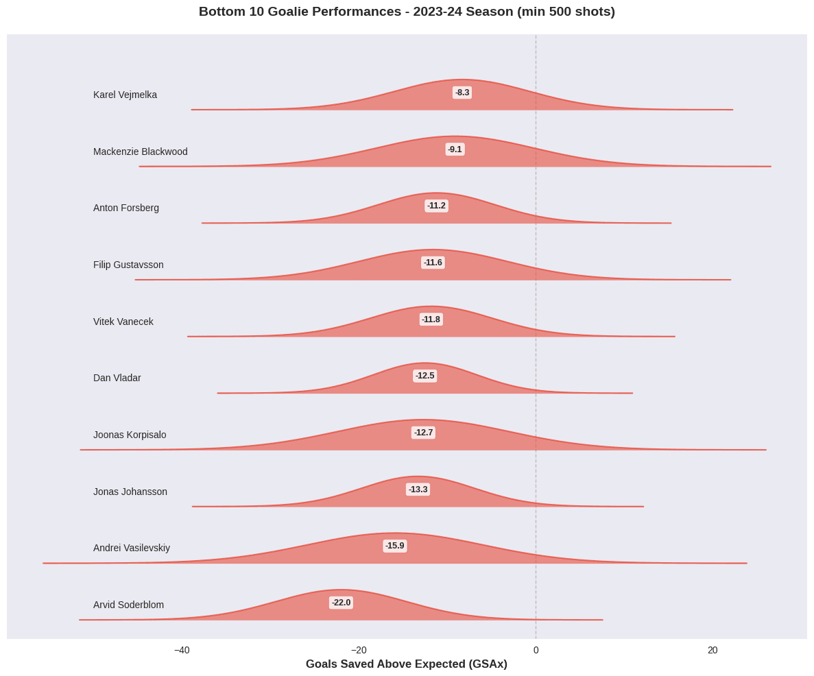
The striking characteristic of these results is the amount of residual uncertainty around the estimates of goalie performance. While some clearly outperform or underperform expectations, many fall within a range where their true skill level is ambiguous under this model. This highlights the challenges of isolating individual performance from context and random chance.
Looking at some individual estimates, the top 10 list includes several of the acknowledged top goaltenders from 2023-24, including the Vezina Trophy winner, Connor Hellebuyck and the save percentage leader, Anthony Stolarz. Andrei Vasilevskiy is conspicuous by his presence in the bottom ten. He is one of the top goalies of his era, but turned in an inconsistent season in 2023-24. This model probably exaggerates his poor performance, however, suggesting that the model could still be improved by incorporating additional contextual factors or improved model structure.
Clearing the Crease
The goal (pun intended) of this post was not to build a production-quality goalie evaluation system, but rather to illustrate how Bayesian spatial models can provide a principled approach for estimating goal expectation. By carefully modeling the spatial distribution of shots and goals and incorporating contextual factors, we can chip away at the confounding factors that obscure our ability to estimate shot quality.
We included, for the sake of simplicity, just one potential confounder. Ideally we would have a more comprehensive model incorporating additional contextual variables, shooter effects, and team defensive contributions. But hopefully the path to model improvement is clear, limited only by data availability and computational resources.
Even blessed with comprehensive and complete data, I don’t recommend starting with a feature-complete model. It is difficult to iterate and debug complex models, and simpler models often reveal the most important patterns. Start small, validate carefully, and build up complexity as needed. For example, the length scale issues that prompted us to implement input warping might not have been obvious in a heavily parameterized model.
GSAx estimates should be viewed as one analytical lens among many, not definitive measures of goalie ability. The uncertainty estimates are the most valuable output—they reveal which performance differences are statistically meaningful and which fall within normal variation. Some goalies with negative GSAx have intervals including zero, preventing us from over-interpreting noise as signal. But perhaps most important, they highlight potential areas of model improvement, warning us against becoming overly confident in our conclusions.